35 min to read
[통계계산] 7. Optimization
Computational Statistics

[통계계산] 7. Optimization
목차
- Computer Arithmetic
- LU decomposition
- Cholesky Decomposition
- QR Decomposition
- Interative Methods
- Non-linear Equations
- Optimization
- Numerical Integration
- Random Number Generation
- Monte Carlo Integration
sessionInfo()
R version 3.6.3 (2020-02-29)
Platform: x86_64-pc-linux-gnu (64-bit)
Running under: Ubuntu 18.04.5 LTS

Matrix products: default
BLAS:   /usr/lib/x86_64-linux-gnu/blas/libblas.so.3.7.1
LAPACK: /usr/lib/x86_64-linux-gnu/lapack/liblapack.so.3.7.1

locale:
 [1] LC_CTYPE=en_US.UTF-8       LC_NUMERIC=C
 [3] LC_TIME=en_US.UTF-8        LC_COLLATE=en_US.UTF-8
 [5] LC_MONETARY=en_US.UTF-8    LC_MESSAGES=en_US.UTF-8
 [7] LC_PAPER=en_US.UTF-8       LC_NAME=C
 [9] LC_ADDRESS=C               LC_TELEPHONE=C
[11] LC_MEASUREMENT=en_US.UTF-8 LC_IDENTIFICATION=C

attached base packages:
[1] stats     graphics  grDevices utils     datasets  methods   base

loaded via a namespace (and not attached):
 [1] fansi_0.5.0       digest_0.6.27     utf8_1.2.1        crayon_1.4.1
 [5] IRdisplay_1.0     repr_1.1.3        lifecycle_1.0.0   jsonlite_1.7.2
 [9] evaluate_0.14     pillar_1.6.1      rlang_0.4.11      uuid_0.1-4
[13] vctrs_0.3.8       ellipsis_0.3.2    IRkernel_1.1      tools_3.6.3
[17] compiler_3.6.3    base64enc_0.1-3   pbdZMQ_0.3-5      htmltools_0.5.1.1
Optimization
Unconstrained optimization
-
Problem \(\min_{\mathbf{x}\in \mathbb{R}^d} f(\mathbf{x})\)
-
Maximization: $\min_{\mathbf{x}\in\mathbb{R}^d} -f(\mathbf{x})$
Golden section search
-
$d=1$.
-
Applicable to functions defined on an interval of the real line.
-
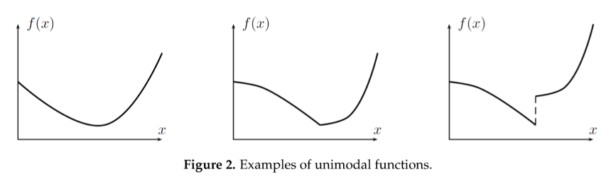
Assumption: $f$ is continuous and unimodal on the interval
-
Idea: keep track of three points $a < x_1 < b$ such that $f(x_1) < \min{f(a), f(b)}$
-
Choose a new point $x_0$ such that $x_0$ belongs to the longer of intervals $(a, x_1)$ and $(x_1, b)$.
-
WLOG, suppose $a < x_0 < x_1$.
- If $f(x_0) > f(x_1)$, then the minimum lies in the interval $(x_0, b)$. Hence set $(a, x_1, b) := (x_0, x_1, b)$.
- If $f(x_0) < f(x_1)$, then the minimum lies in the interval $(a, x_1)$. Hence set $(a, x_1, b) := (a, x_0, x_1)$.
- If $f(x_0) = f(x_1)$, then set $(a, x_1, b) := (x_0, x_1, b)$ if $f(b) < f(a)$, and set $(a, x_1, b) := (a, x_0, x_1)$ otherwise.

-
Above rules do not say how to choose $x_0$. A possibility is to keep the lengths of the two possible candidate intervals the same: $b - x_0 = x_1 - a$, and the relative position of the intermediate points ($x_1$ to $(x_0, b)$; $x_0$ to $(a, x_1)$) the same.
-
Let $\alpha = \frac{x_0 - a}{b - a}$ and $y = \frac{x_1 - x_0}{b -a}$. Then we require $\frac{b - x_1}{b - a} = \alpha$ and \(1:\alpha = y + \alpha : y, \quad \alpha + y + \alpha = 1 .\) By solving this equation, we have $\alpha = \frac{3 - \sqrt{5}}{2}$ or $1 - \alpha = \frac{\sqrt{5} - 1}{2}$, the golden section.

goldensection <- function(f, a, b, tol=1e-6) {
    alpha <- (3 - sqrt(5)) * 0.5
    f
    iter <- 0
    while ( b - a > tol ) {
        x0 <- a + alpha * (b - a)
        x1 <- b - alpha * (b - a)
        print(c(a, x1, b))
        if ( f(x0) > f(x1) ) {
            a <- x0
        } else if ( f(x0) < f(x1) ) {
            b <- x1
            x1 <- x0
        } else {
            if ( f(b) < f(a) ) {
                a <- x0
            } else {
                b <- x1
                x1 <- x0
            }
        }
        iter <- iter + 1
    }
    ret <- list(val = (a + b) / 2, iter = iter)
}
# binomial log-likelihood of 7 successes and 3 failures

F <- function(x) { -7 * log(x) - 3 * log(1 - x) }
goldensection(F, 0.01, 0.99, tol=1e-8)
[1] 0.0100000 0.6156733 0.9900000
[1] 0.3843267 0.7586534 0.9900000
[1] 0.6156733 0.8470199 0.9900000
[1] 0.6156733 0.7586534 0.8470199
[1] 0.6156733 0.7040399 0.7586534
[1] 0.6702868 0.7249004 0.7586534
[1] 0.6702868 0.7040399 0.7249004
[1] 0.6911473 0.7120079 0.7249004
[1] 0.6911473 0.7040399 0.7120079
[1] 0.6911473 0.6991154 0.7040399
[1] 0.6960718 0.7009963 0.7040399
[1] 0.6960718 0.6991154 0.7009963
[1] 0.6979528 0.6998338 0.7009963
[1] 0.6991154 0.7002779 0.7009963
[1] 0.6991154 0.6998338 0.7002779
[1] 0.6995594 0.7000034 0.7002779
[1] 0.6998338 0.7001083 0.7002779
[1] 0.6998338 0.7000034 0.7001083
[1] 0.6999387 0.7000435 0.7001083
[1] 0.6999387 0.7000034 0.7000435
[1] 0.6999787 0.7000187 0.7000435
[1] 0.6999787 0.7000034 0.7000187
[1] 0.6999940 0.7000093 0.7000187
[1] 0.6999940 0.7000034 0.7000093
[1] 0.6999940 0.6999998 0.7000034
[1] 0.6999976 0.7000012 0.7000034
[1] 0.6999976 0.6999998 0.7000012
[1] 0.6999990 0.7000004 0.7000012
[1] 0.6999990 0.6999998 0.7000004
[1] 0.6999995 0.7000000 0.7000004
[1] 0.6999998 0.7000002 0.7000004
[1] 0.6999998 0.7000000 0.7000002
[1] 0.7000000 0.7000001 0.7000002
[1] 0.7000000 0.7000000 0.7000001
[1] 0.7 0.7 0.7
[1] 0.7 0.7 0.7
[1] 0.7 0.7 0.7
[1] 0.7 0.7 0.7
[1] 0.7 0.7 0.7
Convergence of golden section search is slow but sure to find the global minimum (if the assumptions are met).
Newton’s Method
-
First-order optimality condition \(\nabla f(\mathbf{x}^\star) = 0.\)
-
Apply Newton-Raphson to $g(\mathbf{x})=\nabla f(\mathbf{x})$.
-
Idea: iterative quadratic approximation.
-
Second-order Taylor expansion of the objective function around the current iterate $\mathbf{x}^{(t)}$ \(f(\mathbf{x}) \approx f(\mathbf{x}^{(t)}) + \nabla f(\mathbf{x}^{(t)})^T (\mathbf{x} - \mathbf{x}^{(t)}) + \frac {1}{2} (\mathbf{x} - \mathbf{x}^{(t)})^T [\nabla^2 f(\mathbf{x}^{(t)})] (\mathbf{x} - \mathbf{x}^{(t)})\) and then minimize the quadratic approximation.
-
To maximize the quadratic appriximation function, we equate its gradient to zero \(\nabla f(\mathbf{x}^{(t)}) + [\nabla^2 f(\mathbf{x}^{(t)})] (\mathbf{x} - \mathbf{x}^{(t)}) = \mathbf{0},\) which suggests the next iterate \(\begin{eqnarray*} \mathbf{x}^{(t+1)} &=& \mathbf{x}^{(t)} - [\nabla^2 f(\mathbf{x}^{(t)})]^{-1} \nabla f(\mathbf{x}^{(t)}), \end{eqnarray*}\) a complete analogue of the univariate Newton-Raphson for solving $g(x)=0$.
-
Considered the gold standard for its fast (quadratic) convergence: $\mathbf{x}^{(t)} \to \mathbf{x}^{\star}$ and \(\frac{\|\mathbf{x}^{(t+1)} - \mathbf{x}^{\star}\|}{\|\mathbf{x}^{(t)} - \mathbf{x}^{\star}\|^2} \to \text{constant}.\) In words, the estimate gets accurate by two decimal digits per iteration.
We call this naive Newton’s method.
- Stability issue: naive Newton’s iterate is not guaranteed to be a descent algorithm, i.e., that ensures $f(\mathbf{x}^{(t+1)}) \le f(\mathbf{x}^{(t)})$. It’s equally happy to head uphill or downhill. Following example shows that the Newton iterate converges to a local maximum, converges to a local minimum, or diverges depending on starting points.
purenewton <- function(f, df, d2f, x0, maxiter=10, tol=1e-6) {
    xold <- x0
    stop <- FALSE
    iter <- 1
    x <- x0
    while ((!stop) && (iter < maxiter)) {
        x <- x - df(x) / d2f(x)
        print(x)
        xdiff <- x - xold
        if (abs(xdiff) < tol) stop <- TRUE
        xold <- x
        iter <- iter + 1
    }
    return(list(val=x, iter=iter))
}
f <- function(x) sin(x)   # objective function
df <- function(x) cos(x)  # gradient
d2f <- function(x) -sin(x) # hessian
purenewton(f, df, d2f, 2.0)
[1] 1.542342
[1] 1.570804
[1] 1.570796
[1] 1.570796
- $val
- 1.5707963267949
- $iter
- 5

purenewton(f, df, d2f, 2.75)
[1] 0.328211
[1] 3.264834
[1] 11.33789
[1] 10.98155
[1] 10.99558
[1] 10.99557
- $val
- 10.9955742875643
- $iter
- 7

purenewton(f, df, d2f, 4.0)
[1] 4.863691
[1] 4.711224
[1] 4.712389
[1] 4.712389
- $val
- 4.71238898038469
- $iter
- 5

Practical Newton
- A remedy for the instability issue:
- approximate $\nabla^2 f(\mathbf{x}^{(t)})$ by a positive definite $\mathbf{H}^{(t)}$ (if it’s not), and
- line search (backtracking) to ensure the descent property.
-
Why insist on a positive definite approximation of Hessian? First define the Newton direction: \(\Delta \mathbf{x}^{(t)} = [\mathbf{H}^{(t)}]^{-1} \nabla f(\mathbf{x}^{(t)}).\) By first-order Taylor expansion, \(\begin{align*} f(\mathbf{x}^{(t)} + s \Delta \mathbf{x}^{(t)}) - f(\mathbf{x}^{(t)}) &= \nabla f(\mathbf{x}^{(t)})^T s \Delta \mathbf{x}^{(t)} + o(s) \\ &= - s \cdot \nabla f(\mathbf{x}^{(t)})^T [\mathbf{H}^{(t)}]^{-1} \nabla f(\mathbf{x}^{(t)}) + o(s). \end{align*}\) For $s$ sufficiently small, $f(\mathbf{x}^{(t)} + s \Delta \mathbf{x}^{(t)}) - f(\mathbf{x}^{(t)})$ is strictly negative if $\mathbf{H}^{(t)}$ is positive definite.
The quantity ${\nabla f(\mathbf{x}^{(t)})^T [\mathbf{H}^{(t)}]^{-1} \nabla f(\mathbf{x}^{(t)})}^{1/2}$ is termed the Newton decrement. -
In summary, a practical Newton-type algorithm iterates according to \(\boxed{ \mathbf{x}^{(t+1)} = \mathbf{x}^{(t)} - s [\mathbf{H}^{(t)}]^{-1} \nabla f(\mathbf{x}^{(t)}) = \mathbf{x}^{(t)} + s \Delta \mathbf{x}^{(t)} }\) where $\mathbf{H}^{(t)}$ is a positive definite approximation to $\nabla^2 f(\mathbf{x}^{(t)})$ and $s$ is a step size.
- For strictly convex $f$, $\nabla^2 f(\mathbf{x}^{(t)})$ is always positive definite. In this case, the above algorithm is called damped Newton. However, line search is still needed (at least for a finite number of times) to guarantee convergence.
Line search
-
Line search: compute the Newton direction and search $s$ such that $f(\mathbf{x}^{(t)} + s \Delta \mathbf{x}^{(t)})$ is minimized.
-
Note the Newton direction only needs to be calculated once. Cost of line search mainly lies in objective function evaluation.
-
Full line search: $s = \arg\min_{\alpha} f(\mathbf{x}^{(t)} + \alpha \Delta \mathbf{x}^{(t)})$. May use golden section search.
-
Approximate line search: step-halving ($s=1,1/2,\ldots$), Amijo rule, …
-
Backtracking line search (Armijo rule)
  # Backtracking line search
  # given: descent direction ∆x, x ∈ domf, α ∈ (0,0.5), β ∈ (0,1).
  t <- 1.0
  while (f(x + t * delx) > f(x) + alpha * t * sum(gradf(x) * delx) {
      t <- beta * t
  }
![]()
The lower dashed line shows the linear extrapolation of $f$, and the upper dashed line has a slope a factor of α smaller. The backtracking condition is that $f$ lies below the upper dashed line, i.e., $0 \le t \le t_0$.
-
How to approximate $\nabla^2 f(\mathbf{x})$? More of an art than science. Often requires problem specific analysis.
-
Taking $\mathbf{H}^{(t)} = \mathbf{I}$ leads to the gradient descent method (see below).
Fisher scoring
-
Consider MLE in which $f(\mathbf{x}) = -\ell(\boldsymbol{\theta})$, where $\ell(\boldsymbol{\theta})$ is the log-likelihood of parameter $\boldsymbol{\theta}$.
-
Fisher scoring method: replace $- \nabla^2 \ell(\boldsymbol{\theta})$ by the expected Fisher information matrix \(\mathbf{I}(\theta) = \mathbf{E}[-\nabla^2\ell(\boldsymbol{\theta})] = \mathbf{E}[\nabla \ell(\boldsymbol{\theta}) \nabla \ell(\boldsymbol{\theta})^T] \succeq \mathbf{0},\) which is true under exchangeability of tne expectation and the differentiation (true for most common distributions).
Therefore we set $\mathbf{H}^{(t)}=\mathbf{I}(\boldsymbol{\theta}^{(t)})$ and obtain the Fisher scoring algorithm: \(\boxed{ \boldsymbol{\theta}^{(t+1)} = \boldsymbol{\theta}^{(t)} + s [\mathbf{I}(\boldsymbol{\theta}^{(t)})]^{-1} \nabla \ell(\boldsymbol{\theta}^{(t)})}.\)
-
Combined with line search, a descent algorithm can be devised.
Example: logistic regression
-
Binary data: response $y_i \in {0,1}$, predictor $\mathbf{x}_i \in \mathbb{R}^{p}$.
-
Model: $y_i \sim $Bernoulli$(p_i)$, where \begin{eqnarray} \mathbf{E} (y_i) = p_i &=& g^{-1}(\eta_i) = \frac{e^{\eta_i}}{1+ e^{\eta_i}} \quad \text{(mean function, inverse link function)}
\eta_i = \mathbf{x}_i^T \beta &=& g(p_i) = \log \left( \frac{p_i}{1-p_i} \right) \quad \text{(logit link function)}. \end{eqnarray} -
MLE: density \begin{eqnarray} f(y_i|p_i) &=& p_i^{y_i} (1-p_i)^{1-y_i}
&=& e^{y_i \log p_i + (1-y_i) \log (1-p_i)}
&=& \exp\left( y_i \log \frac{p_i}{1-p_i} + \log (1-p_i)\right). \end{eqnarray} - Log likelihood of the data $(y_i,\mathbf{x}i)$, $i=1,\ldots,n$, and its derivatives are
\begin{eqnarray*}
\ell(\beta) &=& \sum{i=1}^n \left[ y_i \log p_i + (1-y_i) \log (1-p_i) \right]
&=& \sum_{i=1}^n \left[ y_i \mathbf{x}i^T \beta - \log (1 + e^{\mathbf{x}_i^T \beta}) \right]
\nabla \ell(\beta) &=& \sum{i=1}^n \left( y_i \mathbf{x}i - \frac{e^{\mathbf{x}_i^T \beta}}{1+e^{\mathbf{x}_i^T \beta}} \mathbf{x}_i \right)
&=& \sum{i=1}^n (y_i - p_i) \mathbf{x}_i = \mathbf{X}^T (\mathbf{y} - \mathbf{p})
- \nabla^2\ell(\beta) &=& \sum_{i=1}^n p_i(1-p_i) \mathbf{x}_i \mathbf{x}_i^T = \mathbf{X}^T \mathbf{W} \mathbf{X}, \quad
\text{where } \mathbf{W} &=& \text{diag}(w_1,\ldots,w_n), w_i = p_i (1-p_i)
\mathbf{I}(\beta) &=& \mathbf{E} [- \nabla^2\ell(\beta)] = \mathbf{X}^T \mathbf{W} \mathbf{X} = - \nabla^2\ell(\beta) \quad \text{!!!} \end{eqnarray*} (why the last line?)
- \nabla^2\ell(\beta) &=& \sum_{i=1}^n p_i(1-p_i) \mathbf{x}_i \mathbf{x}_i^T = \mathbf{X}^T \mathbf{W} \mathbf{X}, \quad
\text{where } \mathbf{W} &=& \text{diag}(w_1,\ldots,w_n), w_i = p_i (1-p_i)
-
Therefore for this problem Newton’s method == Fisher scoring: \(\begin{eqnarray*} \beta^{(t+1)} &=& \beta^{(t)} + s[-\nabla^2 \ell(\beta^{(t)})]^{-1} \nabla \ell(\beta^{(t)}) \\ &=& \beta^{(t)} + s(\mathbf{X}^T \mathbf{W}^{(t)} \mathbf{X})^{-1} \mathbf{X}^T (\mathbf{y} - \mathbf{p}^{(t)}) \\ &=& (\mathbf{X}^T \mathbf{W}^{(t)} \mathbf{X})^{-1} \mathbf{X}^T \mathbf{W}^{(t)} \left[ \mathbf{X} \beta^{(t)} + s(\mathbf{W}^{(t)})^{-1} (\mathbf{y} - \mathbf{p}^{(t)}) \right] \\ &=& (\mathbf{X}^T \mathbf{W}^{(t)} \mathbf{X})^{-1} \mathbf{X}^T \mathbf{W}^{(t)} \mathbf{z}^{(t)}, \end{eqnarray*}\) where \(\mathbf{z}^{(t)} = \mathbf{X} \beta^{(t)} + s[\mathbf{W}^{(t)}]^{-1} (\mathbf{y} - \mathbf{p}^{(t)})\) are the working responses. A Newton iteration is equivalent to solving a weighed least squares problem \(\min_{\beta} \sum_{i=1}^n w_i (z_i - \mathbf{x}_i^T \beta)^2\) for which we know how to solve well. Thus the name IRLS (iteratively re-weighted least squares).
- Implication: if a weighted least squares solver is at hand, then logistic regression models can be fitted.
- IRLS == Fisher scoring == Newton’s method
Example: Poisson regression
-
Count data: response $y_i \in {0, 1, 2, \dotsc }$, predictor $\mathbf{x}_i \in \mathbb{R}^{p}$.
-
Model: $y_i \sim $Poisson$(\lambda_i)$, where \begin{eqnarray} \mathbf{E} (y_i) = \lambda_i &=& g^{-1}(\eta_i) = e^{\eta_i} \quad \text{(mean function, inverse link function)}
\eta_i = \mathbf{x}_i^T \beta &=& g(p_i) = \log \lambda_i \quad \text{(logit link function)}. \end{eqnarray} -
MLE: density \begin{eqnarray} f(y_i|\lambda_i) &=& e^{-\lambda_i}\frac{\lambda_i^{y_i}}{y_i!}
&=& \exp\left( y_i \log \lambda_i - \lambda_i - \log(y_i!) \right) \end{eqnarray} - Log likelihood of the data $(y_i,\mathbf{x}i)$, $i=1,\ldots,n$, and its derivatives are
\begin{eqnarray*}
\ell(\beta) &=& \sum{i=1}^n \left[ y_i \log \lambda_i - \lambda_i - \log(y_i!) \right]
&=& \sum_{i=1}^n \left[ y_i \mathbf{x}i^T \beta - \exp(\mathbf{x}_i^T \beta) - \log(y_i!) \right]
\nabla \ell(\beta) &=& \sum{i=1}^n \left( y_i \mathbf{x}i - \exp(\mathbf{x}_i^T \beta)\mathbf{x}_i \right)
&=& \sum{i=1}^n (y_i - \lambda_i) \mathbf{x}_i = \mathbf{X}^T (\mathbf{y} - \boldsymbol{\lambda})
- \nabla^2\ell(\beta) &=& \sum_{i=1}^n \lambda_i \mathbf{x}_i \mathbf{x}_i^T = \mathbf{X}^T \mathbf{W} \mathbf{X}, \quad
\text{where } \mathbf{W} = \text{diag}(\lambda_1,\ldots,\lambda_n)
\mathbf{I}(\beta) &=& \mathbf{E} [- \nabla^2\ell(\beta)] = \mathbf{X}^T \mathbf{W} \mathbf{X} = - \nabla^2\ell(\beta) \quad \text{!!!} \end{eqnarray*} (why the last line?)
- \nabla^2\ell(\beta) &=& \sum_{i=1}^n \lambda_i \mathbf{x}_i \mathbf{x}_i^T = \mathbf{X}^T \mathbf{W} \mathbf{X}, \quad
\text{where } \mathbf{W} = \text{diag}(\lambda_1,\ldots,\lambda_n)
-
Therefore for this problem Newton’s method == Fisher scoring: \(\begin{eqnarray*} \beta^{(t+1)} &=& \beta^{(t)} + s[-\nabla^2 \ell(\beta^{(t)})]^{-1} \nabla \ell(\beta^{(t)}) \\ &=& \beta^{(t)} + s(\mathbf{X}^T \mathbf{W}^{(t)} \mathbf{X})^{-1} \mathbf{X}^T (\mathbf{y} - \boldsymbol{\lambda}^{(t)}) \\ &=& (\mathbf{X}^T \mathbf{W}^{(t)} \mathbf{X})^{-1} \mathbf{X}^T \mathbf{W}^{(t)} \left[ \mathbf{X} \beta^{(t)} + s(\mathbf{W}^{(t)})^{-1} (\mathbf{y} - \boldsymbol{\lambda}^{(t)}) \right] \\ &=& (\mathbf{X}^T \mathbf{W}^{(t)} \mathbf{X})^{-1} \mathbf{X}^T \mathbf{W}^{(t)} \mathbf{z}^{(t)}, \end{eqnarray*}\) where \(\mathbf{z}^{(t)} = \mathbf{X} \beta^{(t)} + s[\mathbf{W}^{(t)}]^{-1} (\mathbf{y} - \boldsymbol{\lambda}^{(t)})\) are the working responses. A Newton iteration is again equivalent to solving a weighed least squares problem \(\min_{\beta} \sum_{i=1}^n w_i (z_i - \mathbf{x}_i^T \beta)^2\) which leads to the IRLS.
- Implication: if a weighted least squares solver is at hand, then Poisson regression models can be fitted.
- IRLS == Fisher scoring == Newton’s method
# Quarterly count of AIDS deaths in Australia (from Dobson, 1990)
deaths <- c(0, 1, 2, 3, 1, 4, 9, 18, 23, 31, 20, 25, 37, 45)
(quarters <- seq_along(deaths))
<ol class=list-inline><li>1</li><li>2</li><li>3</li><li>4</li><li>5</li><li>6</li><li>7</li><li>8</li><li>9</li><li>10</li><li>11</li><li>12</li><li>13</li><li>14</li></ol>
# Poisson regression using Fisher scoring (IRLS) and step halving
# Model: lambda = exp(beta0 + beta1 * quarter), or deaths ~ quarter
poissonreg <- function(x, y, maxiter=10, tol=1e-6) {
    beta0 <- matrix(0, nrow=2, ncol=1)   # initial point
    betaold <- beta0
    stop <- FALSE
    iter <- 1
    inneriter <- rep(0, maxiter)  # to count no. step halving
    beta <- beta0
    lik <- function(bet) {eta <- bet[1] + bet[2] * x; sum( y * eta - exp(eta) ) } # log-likelihood
    likold <- lik(betaold)
    while ((!stop) && (iter < maxiter)) {
        eta <- beta[1] + x * beta[2]
        w <- exp(eta)  # lambda
        # line search by step halving
        s <- 1.0
        for (i in 1:5) {
            z <- eta + s * (y / w - 1) # working response
            m <- lm(z ~ x, weights=w)  # weighted least squares
            beta <- as.matrix(coef(m))
            curlik <- lik(beta)
            if (curlik > likold) break
            s <- s * 0.5
            inneriter[iter] <- inneriter[iter] + 1
        }
        print(c(as.numeric(beta), inneriter[iter], curlik))
        betadiff <- beta - betaold
        if (norm(betadiff, "F") < tol) stop <- TRUE
        likold <- curlik
        betaold <- beta
        iter <- iter + 1
    }
    return(list(val=as.numeric(beta), iter=iter, inneriter=inneriter[1:iter]))
}
poissonreg(quarters, deaths)
[1]  -1.3076923   0.4184066   3.0000000 443.4763188
[1]   0.6456032   0.2401380   0.0000000 469.9257845
[1]   0.3743785   0.2541525   0.0000000 472.0483495
[1]   0.3400344   0.2564929   0.0000000 472.0625465
[1]   0.3396340   0.2565236   0.0000000 472.0625479
[1]   0.3396339   0.2565236   0.0000000 472.0625479
- $val
-
<ol class=list-inline>
- 0.339633920708135
- 0.256523593717915
</ol> - $iter
- 7
- $inneriter
-
<ol class=list-inline>
- 3
- 0
- 0
- 0
- 0
- 0
- 0
</ol>
m <- glm(deaths ~ quarters, family = poisson())
coef(m)
<dl class=dl-inline><dt>(Intercept)</dt><dd>0.339633920708136</dd><dt>quarters</dt><dd>0.256523593717915</dd></dl>
Homework: repeat this using the Armijo rule.
Generalized Linear Models (GLM)
That IRLS == Fisher scoring == Newton’s method for both logistic and Poisson regression is not a coincidence. Let’s consider a more general class of generalized linear models (GLM).
Exponential families
- Random variable $Y$ belongs to an exponential family if the density
\(p(y|\eta,\phi) = \exp \left\{ \frac{y\eta - b(\eta)}{a(\phi)} + c(y,\phi) \right\}.\)
- $\eta$: natural parameter.
- $\phi>0$: dispersion parameter.
- Mean: $\mu= b’(\eta)$. When $b’(\cdot)$ is invertible, function $g(\cdot)=[b’]^{-1}(\cdot)$ is called the canonical link function.
- Variance $\mathbf{Var}{Y}=b’’(\eta)a(\phi)$.
- For example, if $Y \sim \text{Ber}(\mu)$, then \(p(y|\eta,\phi) = \exp\left( y \log \frac{\mu}{1-\mu} + \log (1-\mu)\right).\) Hence \(\eta = \log \frac{\mu}{1-\mu}, \quad \mu = \frac{e^{\eta}}{1+e^{\eta}}, \quad b(\eta) = -\log (1-\mu) = \log(1+e^{\eta})\) Hence \(b'(\eta) = \frac{e^{\eta}}{1+e^{\eta}} = g^{-1}(\eta).\) as above.
| Family | Canonical Link | Variance Function |
|---|---|---|
| Normal (unit variance) | $\eta=\mu$ | 1 |
| Poisson | $\eta=\log \mu$ | $\mu$ |
| Binomial | $\eta=\log \left(\frac{\mu}{1 - \mu} \right)$ | $\mu (1 - \mu)$ |
| Gamma | $\eta = \mu^{-1}$ | $\mu^2$ |
| Inverse Gaussian | $\eta = \mu^{-2}$ | $\mu^3$ |
Generalized linear models
GLM models the conditional distribution of $Y$ given predictors $\mathbf{x}$ through the conditional mean $\mu = \mathbf{E}(Y|\mathbf{x})$ via a strictly increasing link function \(g(\mu) = \mathbf{x}^T \beta, \quad \mu = g^{-1}(\mathbf{x}^T\beta) = b'(\eta)\)
From these relations we have (assuming no overdispertion, i.e., $a(\phi)\equiv 1$) \(\mathbf{x}^T\beta = g'(\mu)d\mu, \quad d\mu = b''(\eta)d\eta, \quad b''(\eta) = \mathbf{Var}[Y] = \sigma^2, \quad d\eta = \frac{1}{b''(\eta)}d\mu = \frac{1}{b''(\eta)g'(\mu)}\mathbf{x}^T d\beta.\)
Then, after some workout with matrix calculus, we have for $n$ samples:
- Score, Hessian, information
\begin{eqnarray}
\nabla\ell(\beta) &=& \sum_{i=1}^n \frac{(y_i-\mu_i) [1/g’(\mu_i)]}{\sigma^2} \mathbf{x}_i, \quad \mu_i = \mathbf{x}_i^T\beta,
- \nabla^2 \ell(\beta) &=& \sum_{i=1}^n \frac{[1/g’(\mu_i)]^2}{\sigma^2} \mathbf{x}_i \mathbf{x}_i^T - \sum_{i=1}^n \frac{(y_i - \mu_i)[b’’’(\eta_i)/[b’’(\eta_i)g’(\mu_i)]^2+g’’(\mu_i)/[g’(\mu_i)]^3]}{\sigma^2} \mathbf{x}_i \mathbf{x}_i^T, \quad \eta_i = [b’]^{-1}(\eta),
\mathbf{I}(\beta) &=& \mathbf{E} [- \nabla^2 \ell(\beta)] = \sum_{i=1}^n \frac{[1/g’(\mu_i)]^2}{\sigma^2} \mathbf{x}_i \mathbf{x}_i^T = \mathbf{X}^T \mathbf{W} \mathbf{X}.
\end{eqnarray}
-
Fisher scoring method: \(\beta^{(t+1)} = \beta^{(t)} + s [\mathbf{I}(\beta^{(t)})]^{-1} \nabla \ell(\beta^{(t)})\) IRLS with weights $w_i = [1/g’(\mu_i)]^2/\sigma^2$ and some working responses $z_i$.
-
For canonical link, $\mathbf{x}^T\beta = g(\mu) =[b’]^{-1}(\mu) = \eta$. The second term of Hessian vanishes because $d\eta=\mathbf{x}^Td\beta$ and $d^2\eta=0$. The Hessian coincides with Fisher information matrix. IRLS == Fisher scoring == Newton’s method. Hence MLE is a convex optimization problem.
-
Non-canonical link, Fisher scoring != Newton’s method, and MLE is a non-convex optimization problem.
Example: Probit regression (binary response with probit link). \begin{eqnarray} y_i &\sim& \text{Ber}(p_i)
p_i &=& \Phi(\mathbf{x}_i^T \beta)
\eta_i &=& \log\left(\frac{p_i}{1-p_i}\right) \neq \mathbf{x}_i^T \beta = \Phi^{-1}(p_i). \end{eqnarray} where $\Phi(\cdot)$ is the cdf of a standard normal. -
R implements the Fisher scoring method, aka IRLS, for GLMs in function
glm().
Nonlinear regression - Gauss-Newton method
- Now we finally get to the problem Gauss faced in 1801!
Relocate the dwarf planet Ceres https://en.wikipedia.org/wiki/Ceres_(dwarf_planet) by fitting 24 observations to a 6-parameter (nonlinear) orbit.- In 1801, Jan 1 – Feb 11 (41 days), astronomer Piazzi discovered Ceres, which was lost behind the Sun after observing its orbit 24 times.
- Aug – Sep, futile search by top astronomers; Laplace claimed it unsolvable.
- Oct – Nov, Gauss did calculations by method of least squares, sent his results to astronomer von Zach.
- Dec 31, von Zach relocated Ceres according to Gauss’ calculation.
- Nonlinear least squares (curve fitting): \(\text{minimize} \,\, f(\beta) = \frac{1}{2} \sum_{i=1}^n [y_i - \mu_i(\mathbf{x}_i, \beta)]^2\) For example, $y_i =$ dry weight of onion and $x_i=$ growth time, and we want to fit a 3-parameter growth curve \(\mu(x, \beta_1,\beta_2,\beta_3) = \frac{\beta_3}{1 + \exp(-\beta_1 - \beta_2 x)}.\)

-
If $\mu_i$ is a linear function of $\beta$, i.e., $\mathbf{x}_i^T\beta$, then NLLS reduces to the usual least squares.
-
“Score” and “information matrices” \(\begin{eqnarray*} \nabla f(\beta) &=& - \sum_{i=1}^n [y_i - \mu_i(\mathbf{x}_i,\beta)] \nabla \mu_i(\mathbf{x}_i,\beta) \\ \nabla^2 f(\beta) &=& \sum_{i=1}^n \nabla \mu_i(\mathbf{x}_i,\beta) \nabla \mu_i(\mathbf{x}_i,\beta)^T - \sum_{i=1}^n [y_i - \mu_i(\mathbf{x}_i,\beta)] \nabla^2 \mu_i(\mathbf{x}_i,\beta) \\ \mathbf{I}(\beta) &=& \sum_{i=1}^n \nabla \mu_i(\mathbf{x}_i,\beta) \nabla \mu_i(\mathbf{x}_i,\beta)^T = \mathbf{J}(\beta)^T \mathbf{J}(\beta), \end{eqnarray*}\) where $\mathbf{J}(\beta)^T = [\nabla \mu_1(\mathbf{x}_1,\beta), \ldots, \nabla \mu_n(\mathbf{x}_n,\beta)] \in \mathbb{R}^{p \times n}$.
-
Gauss-Newton (= “Fisher scoring method”) uses $\mathbf{I}(\beta)$, which is always positive semidefinite. \(\boxed{ \beta^{(t+1)} = \beta^{(t)} - s [\mathbf{I} (\beta^{(t)})]^{-1} \nabla f(\beta^{(t)}) }\)
- Justification
- Residuals $y_i - \mu_i(\mathbf{x}_i, \beta)$ are small, or $\mu_i$ is nearly linear;
- Model the data as $y_i \sim N(\mu_i(\mathbf{x}i, \beta), \sigma^2)$, where $\sigma^2$ is assumed to be known. Then,
\begin{align*}
\ell(\beta) &= -\frac{1}{2\sigma^2}\sum{i=1}^n [y_i - \mu_i(\beta)] \nabla \mu_i(\mathbf{x}i, \beta)
\nabla\ell(\beta) &= -\sum{i=1}^n \nabla \mu_i(\mathbf{x}i,\beta) \nabla \mu_i(\mathbf{x}_i,\beta)^T - \sum{i=1}^n [y_i - \mu_i(\beta)] \nabla^2 \mu_i(\mathbf{x}i, \beta)
-\nabla^2 \ell(\beta) &= \sum{i=1}^n \nabla \mu_i(\mathbf{x}i,\beta) \nabla \mu_i(\mathbf{x}_i,\beta)^T - \sum{i=1}^n [y_i - \mu_i(\beta)] \nabla^2 \mu_i(\mathbf{x}_i,\beta)
\end{align*} Thus \(\mathbf{E}[-\nabla^2 \ell(\beta)] = \sum_{i=1}^n \nabla \mu_i(\beta) \nabla \mu_i(\beta)^T.\)
- In fact Gauss invented the Gaussian (normal) distribution to justify this method!
Quasi-Newton methods
-
First order Taylor expansion of $\nabla f(\mathbf{x})$ at $\mathbf{x}^{(t)}$ around $\mathbf{x}^{(t+1)}$: \(\nabla f(\mathbf{x}^{(t)}) - \nabla f(\mathbf{x}^{(t+1)}) \approx \nabla^2 f(\mathbf{x}^{(t+1)})(\mathbf{x}^{(t)} - \mathbf{x}^{(t+1)}) .\)
-
Secant condition \(\nabla f(\mathbf{x}^{(t)}) - \nabla f(\mathbf{x}^{(t+1)}) = \mathbf{M}^{(t+1)}(\mathbf{x}^{(t)} - \mathbf{x}^{(t+1)})\) for some sequence of positive definite matrices ${\mathbf{M}^{(t)}}$.

-
Davidon (1959): symmetric rank-1 update formula \(\mathbf{M}^{(t+1)} = \mathbf{M}^{(t)} + c_t\mathbf{v}^{(t)}\mathbf{v}^{(t)T}\) Let $\mathbf{g}^{(t)} = \nabla f(\mathbf{x}^{(t)}) - \nabla f(\mathbf{x}^{(t+1)})$ and $\mathbf{s}^{(t)} = \mathbf{x}^{(t)} - \mathbf{x}^{(t+1)}$. \(\mathbf{g}^{(t)} = (\mathbf{M}^{(t)} + c_t\mathbf{v}^{(t)}\mathbf{v}^{(t)T})\mathbf{s}^{(t)} = \mathbf{M}^{(t)}\mathbf{s}^{(t)} + c_t(\mathbf{v}^{(t)T}\mathbf{s}^{(t)})\mathbf{v}^{(t)}\) suggests a choice (unique up to scaling) \begin{align} \mathbf{v}^{(t)} &= \mathbf{g}^{(t)} - \mathbf{M}^{(t)}\mathbf{s}^{(t)}
c_t &= 1/[(\mathbf{g}^{(t)} - \mathbf{M}^{(t)}\mathbf{s}^{(t)})^T\mathbf{s}^{(t)}] \end{align} -
Positive definiteness of $\mathbf{M}^{(t+1)}$ is guaranteed if $\mathbf{M}^{(t)}$ is PD and $c_t \ge 0$, or $c_t < 0$ and $1 + c_t\mathbf{v}^{(t)}[\mathbf{M}^{(t)}]^{-1}\mathbf{v}^{(t)} > 0$. The latter is because by the Sherman-Morris formula: \([\mathbf{M}^{(t)} + c_t\mathbf{v}^{(t)}\mathbf{v}^{(t)T}]^{-1} = [\mathbf{M}^{(t)}]^{-1} - \frac{c_t}{1 + c_t\mathbf{v}^{(t)}[\mathbf{M}^{(t)}]^{-1}\mathbf{v}}([\mathbf{M}^{(t)}]^{-1}\mathbf{v}^{(t)})([\mathbf{M}^{(t)}]^{-1}\mathbf{v}^{(t)})^T\)
-
Unfortunately, $c_t$ may not be well-defined if $(\mathbf{g}^{(t)} - \mathbf{M}^{(t)}\mathbf{s}^{(t)})^T\mathbf{s}^{(t)} = 0$.
-
A remedy to to switch to the rank-2 update, yielding the Broyden class update rule: \begin{align} \mathbf{M}^{(t+1)} &= \mathbf{M}^{(t)} - \frac{1}{\mathbf{s}^{(t)T}\mathbf{M}^{(t)}\mathbf{s}^{(t)}}\mathbf{M}^{(t)}\mathbf{s}^{(t)}\mathbf{s}^{(t)T}\mathbf{M}^{(t)} + \frac{1}{\mathbf{s}^{(t)T}\mathbf{g}^{(t)}}\mathbf{g}^{(t)}\mathbf{g}^{(t)T} + \phi\mathbf{w}^{(t)}\mathbf{w}^{(t)T},
\mathbf{w}^{(t)} &= (\mathbf{s}^{(t)T}\mathbf{M}^{(t)}\mathbf{s}^{(t)})^{1/2}\left( \frac{1}{\mathbf{s}^{(t)T}\mathbf{g}^{(t)}}\mathbf{g}^{(t)} - \frac{1}{\mathbf{s}^{(t)T}\mathbf{M}^{(t)}\mathbf{s}^{(t)}}\mathbf{M}^{(t)}\mathbf{s}^{(t)} \right) \end{align}- PD is preserved if $\phi \ge 0$;
- Broyden-Fletcher-Goldfarb-Shanno (BFGS): $\phi=0$;
- Davidon-Fletcher-Powell (DFP): $\phi=1$.
-
R’s general-purpose optimization routine
optim()supports BFGS.
Gradient descent method
-
Iteration: \(\boxed{ \mathbf{x}^{(t+1)} = \mathbf{x}^{(t)} - \gamma_t\nabla f(\mathbf{x}^{(t)}) }\) for some step size $\gamma_t$. This is a special case of the Netwon-type algorithms with $\mathbf{H}_t = \mathbf{I}$ and $\Delta\mathbf{x} = \nabla f(\mathbf{x}^{(t)})$.
-
Idea: iterative linear approximation (first-order Taylor series expansion). \(f(\mathbf{x}) \approx f(\mathbf{x}^{(t)}) + \nabla f(\mathbf{x}^{(t)})^T (\mathbf{x} - \mathbf{x}^{(t)})\) and then minimize the linear approximation within a compact set: let $\Delta\mathbf{x} = \mathbf{x}^{(t+1)}-\mathbf{x}^{(t)}$ to choose. Solve \(\min_{\|\Delta\mathbf{x}\|_2 \le 1} \nabla f(\mathbf{x}^{(t)})^T\Delta\mathbf{x}\) to obtain $\Delta\mathbf{x} = -\nabla f(\mathbf{x}^{(t)})/|\nabla f(\mathbf{x}^{(t)})|_2 \propto -\nabla f(\mathbf{x}^{(t)})$.
- Step sizes are chosen so that the descent property is maintained (e.g., line search).
- Step size must be chosen at any time, since unlike Netwon’s method, first-order approximation is always unbounded below.
- Pros
- Each iteration is inexpensive.
- No need to derive, compute, store and invert Hessians; attractive in large scale problems.
- Cons
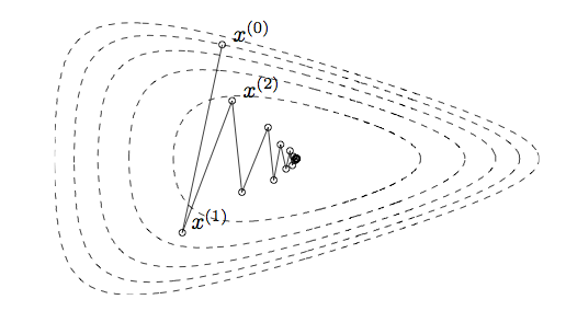
- Slow convergence (zigzagging).
- Do not work for non-smooth problems.
Convergence
-
In general, the best we can obtain from gradient descent is linear convergence (cf. quadratic convergence of Newton).
-
Example \(f(\mathbf{x}) = \frac{1}{2}(x_1^2 + c x_2^2), \quad c > 1\) The optimal value is 0.
It can be shown that if we start from $x^{(0)}=(c, 1)$, then \(f(\mathbf{x}^{(t)}) = \left(\frac{c-1}{c+1}\right)^t f(\mathbf{x}^{(0)})\) and \(\|\mathbf{x}^{(t)} - \mathbf{x}^{\star}\|_2 = \left(\frac{c-1}{c+1}\right)^t \|\mathbf{x}^{(0)} - \mathbf{x}^{\star}\|_2\)
-
More generally, if
- $f$ is convex and differentiable over $\mathbb{R}^d$;
- $f$ has $L$-Lipschitz gradients, i.e., $|\nabla f(\mathbf{x}) - \nabla f(\mathbf{y})|_2 \le L|\mathbf{x} - \mathbf{y} |_2$;
- $p^{\star} = \inf_{\mathbf{x}\in\mathbb{R}^d} f(x) > -\infty$ and attained at $\mathbf{x}^{\star}$,
then \(f(\mathbf{x}^{(t)}) - p^{\star} \le \frac{1}{2\gamma t}\|\mathbf{x}^{(0)} - \mathbf{x}^{\star}\|_2^2 = O(1/t).\) for constant step size ($\gamma_t = \gamma \in (0, 1/L]$), a sublinear convergence. Similar upper bound with line search.
Examples
-
Least squares: $f(\beta) = \frac{1}{2}|\mathbf{X}\beta - \mathbf{y}|_2^2 = \frac{1}{2}\beta^T\mathbf{X}^T\mathbf{X}\beta - \beta^T\mathbf{X}^T\mathbf{y} + \frac{1}{2}\mathbf{y}^T\mathbf{y}$
- Gradient $\nabla f(\beta) = \mathbf{X}^T\mathbf{X}\beta - \mathbf{X}^T\mathbf{y}$ is $|\mathbf{X}^T\mathbf{X}|2$-Lipschitz. Hence $\gamma \in (0, 1/\sigma{\max}(\mathbf{X})^2]$ guarantees descent property and convergence.
-
Logistic regression: $f(\beta) = -\sum_{i=1}^n \left[ y_i \mathbf{x}_i^T \beta - \log (1 + e^{\mathbf{x}_i^T \beta}) \right]$
-
Gradient $\nabla f(\beta) = - \mathbf{X}^T (\mathbf{y} - \mathbf{p})$ is $\frac{1}{4}|\mathbf{X}^T\mathbf{X}|_2$-Lipschitz.
-
May be unbounded below, e.g., all the data are of the same class.
-
Adding a ridge penalty $\frac{\rho}{2}|\beta|_2^2$ makes the problem identifiable.
-
-
Poisson regression: $f(\beta) = -\sum_{i=1}^n \left[ y_i \mathbf{x}_i^T \beta - \exp(\mathbf{x}_i^T \beta) - \log(y_i!) \right]$
- Gradient
\begin{eqnarray}
\nabla f(\beta) &=& -\sum_{i=1}^n \left( y_i \mathbf{x}_i - \exp(\mathbf{x}_i^T \beta)\mathbf{x}_i \right)
&=& -\sum_{i=1}^n (y_i - \lambda_i) \mathbf{x}_i = -\mathbf{X}^T (\mathbf{y} - \boldsymbol{\lambda}) \end{eqnarray} is not Lipschitz (HW). What is the consequence?
- Gradient
\begin{eqnarray}
\nabla f(\beta) &=& -\sum_{i=1}^n \left( y_i \mathbf{x}_i - \exp(\mathbf{x}_i^T \beta)\mathbf{x}_i \right)
# Poisson regression using gradient descent
# Model: lambda = exp(beta0 + beta1 * quarter), or deaths ~ quarter
poissonreg_grad <- function(x, y, maxiter=10, tol=1e-6) {
    beta0 <- matrix(0, nrow=2, ncol=1)   # initial point
    betaold <- beta0
    iter <- 1
    inneriter <- rep(0, maxiter)  # to count no. step halving
    betamat <- matrix(NA, nrow=maxiter, ncol=length(beta0) + 2)
    colnames(betamat) <- c("beta0", "beta1", "inneriter", "lik")
    beta <- beta0
    lik <- function(bet) {eta <- bet[1] + bet[2] * x; sum( y * eta - exp(eta) ) } # log-likelihood
    likold <- lik(betaold)
    while (iter < maxiter) {
        eta <- beta[1] + x * beta[2]
        lam <- exp(eta)  # lambda
        grad <- as.matrix(c(sum(lam - y), sum((lam - y) * x)))
        # line search by step halving
        #s <- 0.00001
        s <- 0.00005
        for (i in 1:5) {
            beta <- beta - s * grad
            curlik <- lik(beta)
            if (curlik > likold) break
            s <- s * 0.5
            inneriter[iter] <- inneriter[iter] + 1
        }
        #print(c(as.numeric(beta), inneriter[iter], curlik))
        betamat[iter,] <- c(as.numeric(beta), inneriter[iter], curlik)
        betadiff <- beta - betaold
        if (norm(betadiff, "F") < tol) break
        likold <- curlik
        betaold <- beta
        iter <- iter + 1
    }
    #return(list(val=as.numeric(beta), iter=iter, inneriter=inneriter[1:iter]))
    return(betamat[1:iter,])
}
# Australian AIDS data from the IRLS example above
pm <- poissonreg_grad(quarters, deaths, tol=1e-8, maxiter=20000)
head(pm, 10)
tail(pm, 10)
| beta0 | beta1 | inneriter | lik |
|---|---|---|---|
| 0.01025000 | 0.1149500 | 0 | 241.3754 |
| 0.01933954 | 0.2178634 | 0 | 423.2101 |
| 0.02505110 | 0.2826001 | 0 | 471.3151 |
| 0.02532401 | 0.2830995 | 0 | 471.3176 |
| 0.02553404 | 0.2828481 | 0 | 471.3190 |
| 0.02577206 | 0.2829335 | 0 | 471.3201 |
| 0.02599725 | 0.2828674 | 0 | 471.3212 |
| 0.02622798 | 0.2828694 | 0 | 471.3222 |
| 0.02645600 | 0.2828408 | 0 | 471.3233 |
| 0.02668501 | 0.2828259 | 0 | 471.3243 |
| beta0 | beta1 | inneriter | lik | |
|---|---|---|---|---|
| [12951,] | 0.3396212 | 0.2565247 | 0 | 472.0625 |
| [12952,] | 0.3396212 | 0.2565247 | 0 | 472.0625 |
| [12953,] | 0.3396212 | 0.2565247 | 0 | 472.0625 |
| [12954,] | 0.3396212 | 0.2565247 | 0 | 472.0625 |
| [12955,] | 0.3396212 | 0.2565247 | 0 | 472.0625 |
| [12956,] | 0.3396212 | 0.2565247 | 0 | 472.0625 |
| [12957,] | 0.3396212 | 0.2565247 | 0 | 472.0625 |
| [12958,] | 0.3396213 | 0.2565247 | 0 | 472.0625 |
| [12959,] | 0.3396213 | 0.2565247 | 0 | 472.0625 |
| [12960,] | 0.3396213 | 0.2565247 | 0 | 472.0625 |
Recall
m <- glm(deaths ~ quarters, family = poisson())
coef(m)
<dl class=dl-inline><dt>(Intercept)</dt><dd>0.339633920708136</dd><dt>quarters</dt><dd>0.256523593717915</dd></dl>
Coordinate descent
- Idea: coordinate-wise minimization is often easier than the full-dimensional minimization \(x_j^{(t+1)} = \arg\min_{x_j} f(x_1^{(t+1)}, \dotsc, x_{j-1}^{(t+1)}, x_j, x_{j+1}^{(t)}, \dotsc, x_d^{(t)})\)

-
Similar to the Gauss-Seidel method for solving linear equations.
-
Block descent: a vector version of coordinate descent \(\mathbf{x}_j^{(t+1)} = \arg\min_{\mathbf{x}_j} f(\mathbf{x}_1^{(t+1)}, \dotsc, \mathbf{x}_{j-1}^{(t+1)}, \mathbf{x}_j, \mathbf{x}_{j+1}^{(t)}, \dotsc, \mathbf{x}_d^{(t)})\)
- Q: why objective value converges?
- A: descent property
- Caution: even if the objective function is convex, coordinate descent may not converge to the global minimum and converge to a suboptimal point.

- Fortunately, if the objective function is convex and differentible, or a sum of differentible convex function and seperable nonsmooth convex function, i.e., \(h(\mathbf{x}) = f(\mathbf{x}) + \sum_{i=1}^d g_i(x_i),\) where $f$ is convex and differentiable and $g_i$ are convex but not necessarily differentiable, then CD converges to the global minimum.
Comments