16 min to read
[통계계산] 3. Cholesky Decomposition
Computational Statistics

[통계계산] 3. Cholesky Decomposition
목차
- Computer Arithmetic
- LU decomposition
- Cholesky Decomposition
- QR Decomposition
- Interative Methods
- Non-linear Equations
- Optimization
- Numerical Integration
- Random Number Generation
- Monte Carlo Integration
sessionInfo()
R version 3.6.3 (2020-02-29)
Platform: x86_64-pc-linux-gnu (64-bit)
Running under: Ubuntu 18.04.5 LTS

Matrix products: default
BLAS:   /usr/lib/x86_64-linux-gnu/blas/libblas.so.3.7.1
LAPACK: /usr/lib/x86_64-linux-gnu/lapack/liblapack.so.3.7.1

locale:
 [1] LC_CTYPE=en_US.UTF-8       LC_NUMERIC=C
 [3] LC_TIME=en_US.UTF-8        LC_COLLATE=en_US.UTF-8
 [5] LC_MONETARY=en_US.UTF-8    LC_MESSAGES=en_US.UTF-8
 [7] LC_PAPER=en_US.UTF-8       LC_NAME=C
 [9] LC_ADDRESS=C               LC_TELEPHONE=C
[11] LC_MEASUREMENT=en_US.UTF-8 LC_IDENTIFICATION=C

attached base packages:
[1] stats     graphics  grDevices utils     datasets  methods   base

other attached packages:
[1] microbenchmark_1.4-6 mvtnorm_1.0-10       Matrix_1.2-17

loaded via a namespace (and not attached):
 [1] lattice_0.20-44   fansi_0.5.0       digest_0.6.27     utf8_1.2.1
 [5] crayon_1.4.1      IRdisplay_1.0     grid_3.6.3        repr_1.1.3
 [9] lifecycle_1.0.0   jsonlite_1.7.2    evaluate_0.14     pillar_1.6.1
[13] rlang_0.4.11      uuid_0.1-4        vctrs_0.3.8       ellipsis_0.3.2
[17] IRkernel_1.1      tools_3.6.3       compiler_3.6.3    base64enc_0.1-3
[21] pbdZMQ_0.3-5      htmltools_0.5.1.1
Required R packages
library(Matrix)
library(mvtnorm)
library(microbenchmark)
Cholesky Decomposition
-
Named after André-Louis Cholesky, 1875-1918.
-
Our mantra 2:
The structure should be exploited whenever possible in solving a problem.
Common structures include: symmetry, positive (semi)definiteness, sparsity, Kronecker product, low rank, …
-
Recall that a matrix $M$ is positive (semi)definite if \(\mathbf{x}^T\mathbf{M}\mathbf{x} > 0 ~(\ge 0), \quad \forall \mathbf{x}\neq\mathbf{0}.\)
-
We can always assume that a postive (semi)definite matrix is symmetric (why?)
-
Example: normal equation \(\mathbf{X}^T \mathbf{X} \beta = \mathbf{X}^T \mathbf{y}\) for linear regression, the coefficient matrix $\mathbf{X}^T \mathbf{X}$ is symmetric and positive semidefinite. How to exploit this structure?
-
Most of time statisticians deal with positive (semi)definite matrices.
Cholesky decomposition
-
Theorem: Let $\mathbf{A} \in \mathbb{R}^{n \times n}$ be symmetric and positive definite. Then $\mathbf{A} = \mathbf{L} \mathbf{L}^T$, where $\mathbf{L}$ is lower triangular with positive diagonal entries and is unique.
Proof (by induction):
If $n=1$, then $0 < a = \sqrt{a}\sqrt{a}$. For $n>1$, the block equation \(\begin{eqnarray*} \begin{bmatrix} a_{11} & \mathbf{a}^T \\ \mathbf{a} & \mathbf{A}_{22} \end{bmatrix} = \begin{bmatrix} \ell_{11} & \mathbf{0}_{n-1}^T \\ \mathbf{b} & \mathbf{L}_{22} \end{bmatrix} \begin{bmatrix} \ell_{11} & \mathbf{b}^T \\ \mathbf{0}_{n-1} & \mathbf{L}_{22}^T \end{bmatrix} \end{eqnarray*}\) entails \(\begin{eqnarray*} a_{11} &=& \ell_{11}^2 \\ \mathbf{a} &=& \ell_{11} \mathbf{b} \\ \mathbf{A}_{22} &=& \mathbf{b} \mathbf{b}^T + \mathbf{L}_{22} \mathbf{L}_{22}^T . \end{eqnarray*}\)
Since $a_{11}>0$ (why?), $\ell_{11}=\sqrt{a_{11}}$ and $\mathbf{b}=a_{11}^{-1/2}\mathbf{a}$ are uniquely determined. $\mathbf{A}{22} - \mathbf{b} \mathbf{b}^T = \mathbf{A}{22} - a_{11}^{-1} \mathbf{a} \mathbf{a}^T$ is positive definite of size $(n-1)\times(n-1)$ because $\mathbf{A}{22}$ is positive definite (why? homework). By induction hypothesis, lower triangular $\mathbf{L}{22}$ such that $\mathbf{A}{22} - \mathbf{b} \mathbf{b}^T = \mathbf{L}{22}^T\mathbf{L}_{22}$ exists and is unique. -
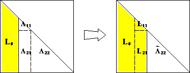
This proof is constructive and completely specifies the algorithm:
for (k in seq_len(n)) {
  for (j in k + seq_len(n - k)) {
      a_jk_div_a_kk <- A[j, k] / A[k, k]
      for (i in j - 1 + seq_len(n - j + 1)) {
          A[i, j] <- A[i, j] - A[i, k] * a_jk_div_a_kk    # L_22
      }
  }
  sqrt_akk <- sqrt(A[k, k])
  for (i in k - 1 + seq_len(n - k + 1)) {
      A[i, k] = A[i, k] / sqrt_akk    # l_11 and b
  }
}

Source: http://www.netlib.org
-
Computational cost: \(\frac{1}{2} [2(n-1)^2 + 2(n-2)^2 + \cdots + 2 \cdot 1^2] \approx \frac{1}{3} n^3 \quad \text{flops}\) plus $n$ square roots. Half the cost of LU decomposition.
-
In general Cholesky decomposition is very stable. Failure of the decomposition simply means $\mathbf{A}$ is not positive definite. It is an efficient way to test positive definiteness.
Pivoting
-
Pivoting is only needed if you want the Cholesky factor of a positive semidefinite matrix.
-
When $\mathbf{A}$ does not have full rank, e.g., $\mathbf{X}^T \mathbf{X}$ with a non-full column rank $\mathbf{X}$, we encounter $a_{kk} = 0$ during the procedure.
-
Symmetric pivoting. At each stage $k$, we permute both row and column such that $\max_{k \le i \le n} a_{ii}$ becomes the pivot. If we encounter $\max_{k \le i \le n} a_{ii} = 0$, then $\mathbf{A}[k:n,k:n] = \mathbf{0}$ (why?) and the algorithm terminates.
-
With symmetric pivoting: \(\mathbf{P} \mathbf{A} \mathbf{P}^T = \mathbf{L} \mathbf{L}^T,\) where $\mathbf{P}$ is a permutation matrix and $\mathbf{L} \in \mathbb{R}^{n \times r}$, $r = \text{rank}(\mathbf{A})$.
Implementation
-
LAPACK functions:
dpotrf(without pivoting),dpstrf(with pivoting). -
R functions:
base::chol()orMatrix::chol()(gives an upper triangular factor: $A = R^T R$)
Example: positive definite matrix
A <- t(Matrix(c(4, 12, -16, 12, 37, -43, -16, -43, 98), nrow=3))  # check out this is pd!
A
3 x 3 Matrix of class "dsyMatrix"
     [,1] [,2] [,3]
[1,]    4   12  -16
[2,]   12   37  -43
[3,]  -16  -43   98
# Cholesky without pivoting
Achol <- Matrix::chol(Matrix::symmpart(A))
Achol
3 x 3 Matrix of class "Cholesky"
     [,1] [,2] [,3]
[1,]    2    6   -8
[2,]    .    1    5
[3,]    .    .    3
class(Achol)
‘Cholesky’
getSlots("Cholesky")
<dl class=dl-inline><dt>x</dt><dd>‘numeric’</dd><dt>Dim</dt><dd>‘integer’</dd><dt>Dimnames</dt><dd>‘list’</dd><dt>uplo</dt><dd>‘character’</dd><dt>diag</dt><dd>‘character’</dd></dl>
str(Achol)
Formal class 'Cholesky' [package "Matrix"] with 5 slots
  ..@ x       : num [1:9] 2 0 0 6 1 0 -8 5 3
  ..@ Dim     : int [1:2] 3 3
  ..@ Dimnames:List of 2
  .. ..$ : NULL
  .. ..$ : NULL
  ..@ uplo    : chr "U"
  ..@ diag    : chr "N"
b <- c(1.0, 2.0, 3.0)
solve(A, b) # this does LU; wasteful!; 2/3 n^3 + 2n^2
3 x 1 Matrix of class "dgeMatrix"
          [,1]
[1,] 28.583333
[2,] -7.666667
[3,]  1.333333
y <- solve(t(Achol), b) # two triangular solves; only 2n^2 flops
solve(Achol, y)
3 x 1 Matrix of class "dgeMatrix"
          [,1]
[1,] 28.583333
[2,] -7.666667
[3,]  1.333333
det(A) # this actually does LU; wasteful!
36.0000000000001
det(Achol)^2 # cheap
36
solve(A) # this does LU!
3 x 3 Matrix of class "dsyMatrix"
           [,1]        [,2]       [,3]
[1,]  49.361111 -13.5555556  2.1111111
[2,] -13.555556   3.7777778 -0.5555556
[3,]   2.111111  -0.5555556  0.1111111
solve(Achol, solve(t(Achol))) # 2n triangular solves
3 x 3 Matrix of class "dgeMatrix"
           [,1]        [,2]       [,3]
[1,]  49.361111 -13.5555556  2.1111111
[2,] -13.555556   3.7777778 -0.5555556
[3,]   2.111111  -0.5555556  0.1111111
Example: positive semidefinite matrix
(A <- Matrix(c(1,1,.5,1,1,.5,.5,.5,1), nrow=3))
eigen(A, symmetric = TRUE)$values
3 x 3 Matrix of class "dsyMatrix"
     [,1] [,2] [,3]
[1,]  1.0  1.0  0.5
[2,]  1.0  1.0  0.5
[3,]  0.5  0.5  1.0
<ol class=list-inline><li>2.36602540378444</li><li>0.633974596215564</li><li>0</li></ol>
Matrix::chol(A, pivot=FALSE) # 2nd argument requests pivoting
Error in asMethod(object): not a positive definite matrix
Traceback:


1. Matrix::chol(A, pivot = FALSE)

2. Matrix::chol(A, pivot = FALSE)

3. .local(x, ...)

4. as(x, if (packed) "dppMatrix" else "dpoMatrix")

5. asMethod(object)

6. stop("not a positive definite matrix")
(Achol <- base::chol(A, pivot=TRUE)) # turn off checking pd
attr(Achol, "pivot")
attr(Achol, "rank")
Warning message in chol.default(A, pivot = TRUE):
“the matrix is either rank-deficient or indefinite”
| 1 | 0.5000000 | 1 |
| 0 | 0.8660254 | 0 |
| 0 | 0.0000000 | 0 |
<ol class=list-inline><li>1</li><li>3</li><li>2</li></ol>
2
Matrix::rankMatrix(A) # determine rank from SVD, which is more numerically stable
2
Achol[, attr(Achol, "pivot")]
| 1 | 1 | 0.5000000 |
| 0 | 0 | 0.8660254 |
| 0 | 0 | 0.0000000 |
(P <- as(attr(Achol, "pivot"), "pMatrix")) # permutation matrix, actually P' in our notation
3 x 3 sparse Matrix of class "pMatrix"

[1,] | . .
[2,] . . |
[3,] . | .
# P A P' = L U
Matrix::norm(t(P) %*% A %*% P - t(Achol) %*% Achol, type="F")  # Frobenius norm
1.11022302462516e-16
Applications
- No inversion principle: whenever we see matrix inverse, we should think in terms of solving linear equations. If the matrix is positive (semi)definite, use Cholesky decomposition, which is twice cheaper than LU decomposition.
Multivariate normal density
Multivariate normal density $\mathcal{N}(0, \Sigma)$, where $\Sigma$ is $n\times n$ positive definite, is \(\frac{1}{(2\pi)^{n/2}\det(\Sigma)^{1/2}}\exp\left(-\frac{1}{2}\mathbf{y}^T\Sigma^{-1}\mathbf{y}\right).\)
Hence the log likelihood is $$
-
\frac{n}{2} \log (2\pi) - \frac{1}{2} \log \det \Sigma - \frac{1}{2} \mathbf{y}^T \Sigma^{-1} \mathbf{y}. $$
- Method 1:
- compute explicit inverse $\Sigma^{-1}$ ($2n^3$ flops),
- compute quadratic form ($2n^2 + 2n$ flops),
- compute determinant ($2n^3/3$ flops).
- Method 2:
- Cholesky decomposition $\Sigma = \mathbf{L} \mathbf{L}^T$ ($n^3/3$ flops),
- Solve $\mathbf{L} \mathbf{x} = \mathbf{y}$ by forward substitutions ($n^2$ flops),
- compute quadratic form $\mathbf{x}^T \mathbf{x}$ ($2n$ flops), and (d) compute determinant from Cholesky factor ($n$ flops).
Which method is better?
# word-by-word transcription of mathematical expression
# Matrix::determinant computes the logarithm of the determinant
logpdf_mvn_1 <- function(y, Sigma) {
    n <- length(y)
    - (n / 2) * log(2 * pi) - (1 / 2) * Matrix::determinant(Sigma)$modulus - (1 / 2) * t(y) %*% solve(Sigma) %*% y
}

# you learnt why you should avoid inversion
logpdf_mvn_2 <- function(y, Sigma) {
    n <- length(y)
    Sigmachol <- Matrix::chol(Matrix::symmpart(Sigma))
    - (n / 2) * log(2 * pi) - Matrix::determinant(Sigmachol)$modulus - (1 / 2) * sum(y * solve(Sigma, y))
}

# this is for the efficiency-concerned
logpdf_mvn_3 <- function(y, Sigma) {
    n <- length(y)
    Sigmachol <- Matrix::chol(Matrix::symmpart(Sigma))
    - 0.5 * n * log(2 * pi) - sum(log(diag(Sigmachol))) - 0.5 * sum(abs(solve(t(Sigmachol), y))^2)
}
set.seed(123) # seed

n <- 1000
# a pd matrix
Sigma_half <- Matrix(rnorm(n * (2 * n)), nrow=n)
Sigma <- Sigma_half %*% t(Sigma_half)
Sigma <- Matrix::symmpart(Sigma)
Sigmachol <- Matrix::chol(Sigma)

y <- Sigmachol %*% rnorm(n)  # one random sample from N(0, Sigma). Homework

# at least they give same answer
(logpdf_mvn_1(y, Sigma))
(logpdf_mvn_2(y, Sigma))
(logpdf_mvn_3(y, Sigma))
1 x 1 Matrix of class "dgeMatrix"
          [,1]
[1,] -5272.565
-5272.56471529637
-5272.56471529637
res <- microbenchmark::microbenchmark(logpdf_mvn_1(y, Sigma), logpdf_mvn_2(y, Sigma), logpdf_mvn_3(y, Sigma))
print(res)
Unit: milliseconds
                   expr      min       lq     mean   median       uq      max
 logpdf_mvn_1(y, Sigma) 405.5765 416.8209 442.0820 425.4402 441.0190 572.9140
 logpdf_mvn_2(y, Sigma) 164.7256 168.7226 178.1795 171.7639 176.7348 307.7929
 logpdf_mvn_3(y, Sigma) 169.3317 176.3511 188.6951 180.4394 191.4759 311.4974
 neval cld
   100   b
   100  a
   100  a
- To evaluate same multivariate normal density at many observations $y_1, y_2, \ldots$, we pre-compute the Cholesky decomposition ($n^3/3$ flops), then each evaluation costs $n^2$ flops.
Linear regression by Cholesky
- Cholesky decomposition is one approach to solve linear regression. Assume $\mathbf{X} \in \mathbb{R}^{n \times p}$ and $\mathbf{y} \in \mathbb{R}^n$.
- Compute $\mathbf{X}^T \mathbf{X}$: $np^2$ flops
- Compute $\mathbf{X}^T \mathbf{y}$: $2np$ flops
- Cholesky decomposition of $\mathbf{X}^T \mathbf{X}$: $\frac{1}{3} p^3$ flops
- Solve normal equation $\mathbf{X}^T \mathbf{X} \beta = \mathbf{X}^T \mathbf{y}$: $2p^2$ flops
- If need standard errors, another $(4/3)p^3$ flops
Total computational cost is $np^2 + (1/3) p^3$ (without s.e.) or $np^2 + (5/3) p^3$ (with s.e.) flops.

Comments