26 min to read
[통계계산] 4. QR Decomposition
Computational Statistics

[통계계산] 4. QR Decomposition
목차
- Computer Arithmetic
- LU decomposition
- Cholesky Decomposition
- QR Decomposition
- Interative Methods
- Non-linear Equations
- Optimization
- Numerical Integration
- Random Number Generation
- Monte Carlo Integration
sessionInfo()
R version 3.6.3 (2020-02-29)
Platform: x86_64-pc-linux-gnu (64-bit)
Running under: Ubuntu 18.04.5 LTS

Matrix products: default
BLAS:   /usr/lib/x86_64-linux-gnu/blas/libblas.so.3.7.1
LAPACK: /usr/lib/x86_64-linux-gnu/lapack/liblapack.so.3.7.1

locale:
 [1] LC_CTYPE=en_US.UTF-8       LC_NUMERIC=C
 [3] LC_TIME=en_US.UTF-8        LC_COLLATE=en_US.UTF-8
 [5] LC_MONETARY=en_US.UTF-8    LC_MESSAGES=en_US.UTF-8
 [7] LC_PAPER=en_US.UTF-8       LC_NAME=C
 [9] LC_ADDRESS=C               LC_TELEPHONE=C
[11] LC_MEASUREMENT=en_US.UTF-8 LC_IDENTIFICATION=C

attached base packages:
[1] stats     graphics  grDevices utils     datasets  methods   base

loaded via a namespace (and not attached):
 [1] fansi_0.5.0       digest_0.6.27     utf8_1.2.1        crayon_1.4.1
 [5] IRdisplay_1.0     repr_1.1.3        lifecycle_1.0.0   jsonlite_1.7.2
 [9] evaluate_0.14     pillar_1.6.1      rlang_0.4.11      uuid_0.1-4
[13] vctrs_0.3.8       ellipsis_0.3.2    IRkernel_1.1      tools_3.6.3
[17] compiler_3.6.3    base64enc_0.1-3   pbdZMQ_0.3-5      htmltools_0.5.1.1
Required R packages
library(Matrix)
QR Decomposition
-
We learned Cholesky decomposition as one approach for solving linear regression.
-
Another approach for linear regression uses the QR decomposition.
This is how thelm()function in R does linear regression.
set.seed(2020) # seed

n <- 5
p <- 3
(X <- matrix(rnorm(n * p), nrow=n)) # predictor matrix
(y <- rnorm(n))    # response vector

# find the (minimum L2 norm) least squares solution
lm(y ~ X - 1)
| 0.3769721 | 0.7205735 | -0.8531228 |
| 0.3015484 | 0.9391210 | 0.9092592 |
| -1.0980232 | -0.2293777 | 1.1963730 |
| -1.1304059 | 1.7591313 | -0.3715839 |
| -2.7965343 | 0.1173668 | -0.1232602 |
<ol class=list-inline><li>1.80004311672545</li><li>1.70399587729432</li><li>-3.03876460529759</li><li>-2.28897494991878</li><li>0.0583034949929225</li></ol>
Call:
lm(formula = y ~ X - 1)

Coefficients:
       X1         X2         X3
 0.615118  -0.008382  -0.770116
We want to understand what is QR and how it is used for solving least squares problem.
Definitions
-
Assume $\mathbf{X} \in \mathbb{R}^{n \times p}$ has full column rank. Necessarilly $n \ge p$.
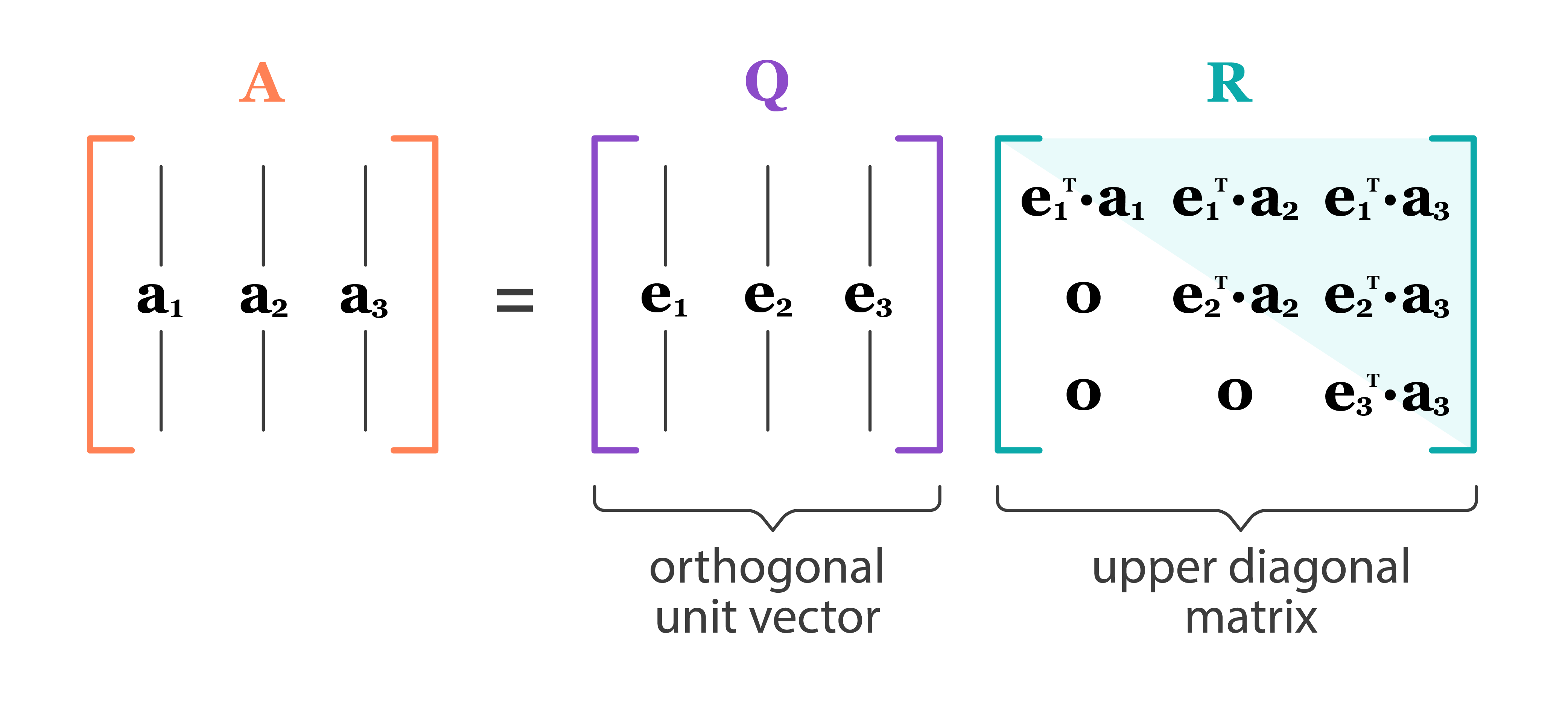
- Full QR decomposition:
\(\mathbf{X} = \mathbf{Q} \mathbf{R},\) where- $\mathbf{Q} \in \mathbb{R}^{n \times n}$, $\mathbf{Q}^T \mathbf{Q} = \mathbf{Q}\mathbf{Q}^T = \mathbf{I}_n$. In other words, $\mathbf{Q}$ is an orthogonal matrix.
- First $p$ columns of $\mathbf{Q}$ form an orthonormal basis of ${\cal R}(\mathbf{X})$ (range or column space of $\mathbf{X}$)
- Last $n-p$ columns of $\mathbf{Q}$ form an orthonormal basis of ${\cal N}(\mathbf{X}^T)$ (null space of $\mathbf{X}^T$)
- Recall that $\mathcal{N}(\mathbf{X}^T)=\mathcal{R}(\mathbf{X})^{\perp}$ and $\mathcal{R}(\mathbf{X}) \oplus \mathcal{N}(\mathbf{X}^T) = \mathbb{R}^n$.
- $\mathbf{R} \in \mathbb{R}^{n \times p}$ is upper triangular with positive diagonal entries.
- The lower $(n-p)\times p$ block of $\mathbf{R}$ is $\mathbf{0}$ (why?).
- $\mathbf{Q} \in \mathbb{R}^{n \times n}$, $\mathbf{Q}^T \mathbf{Q} = \mathbf{Q}\mathbf{Q}^T = \mathbf{I}_n$. In other words, $\mathbf{Q}$ is an orthogonal matrix.
- Reduced QR decomposition:
\(\mathbf{X} = \mathbf{Q}_1 \mathbf{R}_1,\)
where
- $\mathbf{Q}_1 \in \mathbb{R}^{n \times p}$, $\mathbf{Q}_1^T \mathbf{Q}_1 = \mathbf{I}_p$. In other words, $\mathbf{Q}_1$ is a partially orthogonal matrix. Note $\mathbf{Q}_1\mathbf{Q}_1^T \neq \mathbf{I}_n$.
- $\mathbf{R}_1 \in \mathbb{R}^{p \times p}$ is an upper triangular matrix with positive diagonal entries.
- Given QR decomposition $\mathbf{X} = \mathbf{Q} \mathbf{R}$,
\(\mathbf{X}^T \mathbf{X} = \mathbf{R}^T \mathbf{Q}^T \mathbf{Q} \mathbf{R} = \mathbf{R}^T \mathbf{R} = \mathbf{R}_1^T \mathbf{R}_1.\)
- Once we have a (reduced) QR decomposition of $\mathbf{X}$, we automatically have the Cholesky decomposition of the Gram matrix $\mathbf{X}^T \mathbf{X}$.
Least squares
-
Normal equation \(\mathbf{X}^T\mathbf{X}\beta = \mathbf{X}^T\mathbf{y}\) is equivalently written with reduced QR as \(\mathbf{R}_1^T\mathbf{R}_1\beta = \mathbf{R}_1^T\mathbf{Q}_1^T\mathbf{y}\)
-
Since $\mathbf{R}_1$ is invertible, we only need to solve the triangluar system \(\mathbf{R}_1\beta = \mathbf{Q}_1^T\mathbf{y}\) Multiplication $\mathbf{Q}_1^T \mathbf{y}$ is done implicitly (see below).
-
This method is numerically more stable than directly solving the normal equation, since $\kappa(\mathbf{X}^T\mathbf{X}) = \kappa(\mathbf{X})^2$!
-
In case we need standard errors, compute inverse of $\mathbf{R}_1^T \mathbf{R}_1$. This involves triangular solves.
Gram-Schmidt procedure
- Wait! Does $\mathbf{X}$ always have a QR decomposition?
- Yes. It is equivalent to the Gram-Schmidt procedure for basis orthonormalization.
-
Assume $\mathbf{X} = [\mathbf{x}_1 \dotsb \mathbf{x}_p] \in \mathbb{R}^{n \times p}$ has full column rank. That is, $\mathbf{x}_1,\ldots,\mathbf{x}_p$ are linearly independent. -
Gram-Schmidt (GS) procedure produces nested orthonormal basis vectors ${\mathbf{q}1, \dotsc, \mathbf{q}_p}$ that spans $\mathcal{R}(\mathbf{X})$, i.e., \(\begin{split} \text{span}(\{\mathbf{x}_1\}) &= \text{span}(\{\mathbf{q}_1\}) \\ \text{span}(\{\mathbf{x}_1, \mathbf{x}_2\}) &= \text{span}(\{\mathbf{q}_1, \mathbf{q}_2\}) \\ & \vdots \\ \text{span}(\{\mathbf{x}_1, \mathbf{x}_2, \dotsc, \mathbf{x}_p\}) &= \text{span}(\{\mathbf{q}_1, \mathbf{q}_2, \dotsc, \mathbf{q}_p\}) \end{split}\) and $\langle \mathbf{q}_i, \mathbf{q}_j \rangle = \delta{ij}$.
- The algorithm:
- Initialize $\mathbf{q}_1 = \mathbf{x}_1 / |\mathbf{x}_1|_2$
- For $k=2, \ldots, p$, \(\begin{eqnarray*} \mathbf{v}_k &=& \mathbf{x}_k - P_{\text{span}(\{\mathbf{q}_1,\ldots,\mathbf{q}_{k-1}\})}(\mathbf{x}_k) = \mathbf{x}_k - \sum_{j=1}^{k-1} \langle \mathbf{q}_j, \mathbf{x}_k \rangle \cdot \mathbf{q}_j \\ \mathbf{q}_k &=& \mathbf{v}_k / \|\mathbf{v}_k\|_2 \end{eqnarray*}\)
GS conducts reduced QR
-
$\mathbf{Q} = [\mathbf{q}_1 \dotsb \mathbf{q}_p]$. Obviously $\mathbf{Q}^T \mathbf{Q} = \mathbf{I}_p$. - Where is $\mathbf{R}$?
- Let $r_{jk} = \langle \mathbf{q}j, \mathbf{x}_k \rangle$ for $j < k$, and $r{kk} = |\mathbf{v}_k|_2$.
- Re-write the above expression: \(r_{kk} \mathbf{q}_k = \mathbf{x}_k - \sum_{j=1}^{k-1} r_{jk} \cdot \mathbf{q}_j\) or \(\mathbf{x}_k = r_{kk} \mathbf{q}_k + \sum_{j=1}^{k-1} r_{jk} \cdot \mathbf{q}_j .\)
- If we let $r_{jk} = 0$ for $j > k$, then $\mathbf{R}=(r_{jk})$ is upper triangular and \(\mathbf{X} = \mathbf{Q}\mathbf{R} .\)
Source: https://dsc-spidal.github.io/harp/docs/harpdaal/algorithms/
Classical Gram-Schmidt
cgs <- function(X) {  # not in-place
    n <- dim(X)[1]
    p <- dim(X)[2]
    Q <- Matrix(0, nrow=n, ncol=p, sparse=FALSE)
    R <- Matrix(0, nrow=p, ncol=p, sparse=FALSE)
    for (j in seq_len(p)) {
        Q[, j] <- X[, j]
        for (i in seq_len(j-1)) {
            R[i, j] = sum(Q[, i] * X[, j])  # dot product
            Q[, j] <- Q[, j] - R[i, j] * Q[, i]
        }
        R[j, j] <- Matrix::norm(Q[, j, drop=FALSE], "F")
        Q[, j] <- Q[, j] / R[j, j]
    }
    list(Q=Q, R=R)
}
- CGS is unstable (we lose orthogonality due to roundoff errors) when columns of $\mathbf{X}$ are almost collinear.
e <- .Machine$double.eps
(A <- t(Matrix(c(1, 1, 1, e, 0, 0, 0, e, 0, 0, 0, e), nrow=3)))
4 x 3 Matrix of class "dgeMatrix"
             [,1]         [,2]         [,3]
[1,] 1.000000e+00 1.000000e+00 1.000000e+00
[2,] 2.220446e-16 0.000000e+00 0.000000e+00
[3,] 0.000000e+00 2.220446e-16 0.000000e+00
[4,] 0.000000e+00 0.000000e+00 2.220446e-16
res <- cgs(A)
res$Q
4 x 3 Matrix of class "dgeMatrix"
             [,1]       [,2]       [,3]
[1,] 1.000000e+00  0.0000000  0.0000000
[2,] 2.220446e-16 -0.7071068 -0.7071068
[3,] 0.000000e+00  0.7071068  0.0000000
[4,] 0.000000e+00  0.0000000  0.7071068
with(res, t(Q) %*% Q)
3 x 3 Matrix of class "dgeMatrix"
              [,1]          [,2]          [,3]
[1,]  1.000000e+00 -1.570092e-16 -1.570092e-16
[2,] -1.570092e-16  1.000000e+00  5.000000e-01
[3,] -1.570092e-16  5.000000e-01  1.000000e+00
Qis hardly orthogonal.- Where exactly does the problem occur? (HW)
Modified Gram-Schmidt
- The algorithm:
- Initialize $\mathbf{q}_1 = \mathbf{x}_1 / |\mathbf{x}_1|_2$
- For $k=2, \ldots, p$, \(\begin{eqnarray*} \mathbf{v}_k &=& \mathbf{x}_k - P_{\text{span}(\{\mathbf{q}_1,\ldots,\mathbf{q}_{k-1}\})}(\mathbf{x}_k) = \mathbf{x}_k - \sum_{j=1}^{k-1} \langle \mathbf{q}_j, \mathbf{x}_k \rangle \cdot \mathbf{q}_j \\ &=& \mathbf{x}_k - \sum_{j=1}^{k-1} \left\langle \mathbf{q}_j, \mathbf{x}_k - \sum_{l=1}^{j-1}\langle \mathbf{q}_l, \mathbf{x}_k \rangle \mathbf{q}_l \right\rangle \cdot \mathbf{q}_j \\ \mathbf{q}_k &=& \mathbf{v}_k / \|\mathbf{v}_k\|_2 \end{eqnarray*}\)
mgs <- function(X) { # not in-place
    n <- dim(X)[1]
    p <- dim(X)[2]
    R <- Matrix(0, nrow=p, ncol=p)
    for (j in seq_len(p)) {
        for (i in seq_len(j-1)) {
            R[i, j] <- sum(X[, i] * X[, j])  # dot product
            X[, j] <- X[, j] - R[i, j] * X[, i]
        }
        R[j, j] <- Matrix::norm(X[, j, drop=FALSE], "F")
        X[, j] <- X[, j] / R[j, j]
    }
    list(Q=X, R=R)
}
- $\mathbf{X}$ is overwritten by $\mathbf{Q}$ and $\mathbf{R}$ is stored in a separate array.
mres <- mgs(A)
mres$Q
4 x 3 Matrix of class "dgeMatrix"
             [,1]       [,2]       [,3]
[1,] 1.000000e+00  0.0000000  0.0000000
[2,] 2.220446e-16 -0.7071068 -0.4082483
[3,] 0.000000e+00  0.7071068 -0.4082483
[4,] 0.000000e+00  0.0000000  0.8164966
with(mres, t(Q) %*% Q)
3 x 3 Matrix of class "dgeMatrix"
              [,1]          [,2]          [,3]
[1,]  1.000000e+00 -1.570092e-16 -9.064933e-17
[2,] -1.570092e-16  1.000000e+00  1.110223e-16
[3,] -9.064933e-17  1.110223e-16  1.000000e+00
- So MGS is more stable than CGS. However, even MGS is not completely immune to instability.
(B <- t(Matrix(c(0.7, 1/sqrt(2), 0.7 + e, 1/sqrt(2)), nrow=2)))
2 x 2 Matrix of class "dgeMatrix"
     [,1]      [,2]
[1,]  0.7 0.7071068
[2,]  0.7 0.7071068
mres2 <- mgs(B)
mres2$Q
2 x 2 Matrix of class "dgeMatrix"
          [,1] [,2]
[1,] 0.7071068    1
[2,] 0.7071068    0
with(mres2, t(Q) %*% Q)
2 x 2 Matrix of class "dgeMatrix"
          [,1]      [,2]
[1,] 1.0000000 0.7071068
[2,] 0.7071068 1.0000000
Qis hardly orthogonal.-
Where exactly does the problem occur? (HW)
-
Computational cost of CGS and MGS is $\sum_{k=1}^p 4n(k-1) \approx 2np^2$.
-
There are 3 algorithms to compute QR: (modified) Gram-Schmidt, Householder transform, (fast) Givens transform.
In particular, the Householder transform for QR is implemented in LAPACK and thus used in R, Matlab, and Julia.
QR by Householder transform

Alston Scott Householder (1904-1993)
-
This is the algorithm for solving linear regression in R.
-
Assume again $\mathbf{X} = [\mathbf{x}_1 \dotsb \mathbf{x}_p] \in \mathbb{R}^{n \times p}$ has full column rank. -
Gram-Schmidt can be understood as: \(\mathbf{X}\mathbf{R}_{1} \mathbf{R}_2 \cdots \mathbf{R}_n = \mathbf{Q}_1\) where $\mathbf{R}_j$ are a sequence of upper triangular matrices.
-
Householder QR does \(\mathbf{H}_{p} \cdots \mathbf{H}_2 \mathbf{H}_1 \mathbf{X} = \begin{pmatrix} \mathbf{R}_1 \\ \mathbf{0} \end{pmatrix},\) where $\mathbf{H}_j \in \mathbf{R}^{n \times n}$ are a sequence of Householder transformation matrices.
It yields the full QR where $\mathbf{Q} = \mathbf{H}_1 \cdots \mathbf{H}_p \in \mathbb{R}^{n \times n}$. Recall that CGS/MGS only produces the reduced QR decomposition.
- For arbitrary $\mathbf{v}, \mathbf{w} \in \mathbb{R}^{n}$ with $|\mathbf{v}|_2 = |\mathbf{w}|_2$, we can construct a Householder matrix (or Householder reflector) \(\mathbf{H} = \mathbf{I}_n - 2 \mathbf{u} \mathbf{u}^T, \quad \mathbf{u} = - \frac{1}{\|\mathbf{v} - \mathbf{w}\|_2} (\mathbf{v} - \mathbf{w}),\) that transforms $\mathbf{v}$ to $\mathbf{w}$: \(\mathbf{H} \mathbf{v} = \mathbf{w}.\) $\mathbf{H}$ is symmetric and orthogonal. Calculation of Householder vector $\mathbf{u}$ costs $4n$ flops for general $\mathbf{u}$ and $\mathbf{w}$.

-
Now choose $\mathbf{H}_1$ so that \(\mathbf{H}_1 \mathbf{x}_1 = \begin{pmatrix} \|\mathbf{x}_{1}\|_2 \\ 0 \\ \vdots \\ 0 \end{pmatrix}.\) That is, $\mathbf{v} = \mathbf{x}_1$ and $\mathbf{w} = |\mathbf{x}_1|_2\mathbf{e}_1$.
-
Left-multiplying $\mathbf{H}_1$ zeros out the first column of $\mathbf{X}$ below (1, 1).
-
Take $\mathbf{H}_2$ to zero the second column below diagonal: \(\mathbf{H}_2\mathbf{H}_1\mathbf{X} = \begin{bmatrix} \times & \times & \times & \times \\ 0 & \boldsymbol{\times} & \boldsymbol{\times} & \boldsymbol{\times} \\ 0 & \mathbf{0} & \boldsymbol{\times} & \boldsymbol{\times} \\ 0 & \mathbf{0} & \boldsymbol{\times} & \boldsymbol{\times} \\ 0 & \mathbf{0} & \boldsymbol{\times} & \boldsymbol{\times} \end{bmatrix}\)
-
In general, choose the $j$-th Householder transform $\mathbf{H}_j = \mathbf{I}_n - 2 \mathbf{u}_j \mathbf{u}_j^T$, where \(\mathbf{u}_j = \begin{bmatrix} \mathbf{0}_{j-1} \\ {\tilde u}_j \end{bmatrix}, \quad {\tilde u}_j \in \mathbb{R}^{n-j+1},\) to zero the $j$-th column below diagonal. $\mathbf{H}_j$ takes the form \(\mathbf{H}_j = \begin{bmatrix} \mathbf{I}_{j-1} & \\ & \mathbf{I}_{n-j+1} - 2 {\tilde u}_j {\tilde u}_j^T \end{bmatrix} = \begin{bmatrix} \mathbf{I}_{j-1} & \\ & {\tilde H}_{j} \end{bmatrix}.\)
-
Applying a Householder transform $\mathbf{H} = \mathbf{I} - 2 \mathbf{u} \mathbf{u}^T$ to a matrix $\mathbf{X} \in \mathbb{R}^{n \times p}$ \(\mathbf{H} \mathbf{X} = \mathbf{X} - 2 \mathbf{u} (\mathbf{u}^T \mathbf{X})\) costs $4np$ flops. Householder updates never entails explicit formation of the Householder matrices.
-
Note applying ${\tilde H}_j$ to $\mathbf{X}$ only needs $4(n-j+1)(p-j+1)$ flops.
Algorithm
for (j in seq_len(p)) {  # in-place
    u <- Householer(X[j:n, j])
    for (i in j - 1 + seq_len(max(p - j + 1, 0))
        X[j:n, j:p] <- X[j:n, j:p] - 2 * u * sum(u * X[j:n, j:p])
    }
}
-
The process is done in place. Upper triangular part of $\mathbf{X}$ is overwritten by $\mathbf{R}1$ and the essential Householder vectors ($\tilde u{j1}$ is normalized to 1) are stored in $\mathbf{X}[j:n,j]$.
- At $j$-th stage
- computing the Householder vector ${\tilde u}_j$ costs $3(n-j+1)$ flops
- applying the Householder transform ${\tilde H}_j$ to the $\mathbf{X}[j:n, j:p]$ block costs $4(n-j+1)(p-j+1)$ flops
-
In total we need $\sum_{j=1}^p [3(n-j+1) + 4(n-j+1)(p-j+1)] \approx 2np^2 - \frac 23 p^3$ flops.
- Where is $\mathbf{Q}$?
- $\mathbf{Q} = \mathbf{H}_1 \cdots \mathbf{H}_p$. In some applications, it’s necessary to form the orthogonal matrix $\mathbf{Q}$.
Accumulating $\mathbf{Q}$ costs another $2np^2 - \frac 23 p^3$ flops.
-
When computing $\mathbf{Q}^T \mathbf{v}$ or $\mathbf{Q} \mathbf{v}$ as in some applications (e.g., solve linear equation using QR), no need to form $\mathbf{Q}$. Simply apply Householder transforms successively to the vector $\mathbf{v}$. (HW)
- Computational cost of Householder QR for linear regression: $2n p^2 - \frac 23 p^3$ (regression coefficients and $\hat \sigma^2$) or more (fitted values, s.e., …).
Implementation
-
R function:
qr -
Wraps LAPACK routine
dgeqp3(withLAPACK=TRUE; default uses LINPACK, an ancient version of LAPACK).
X  # to recall
y
| 0.3769721 | 0.7205735 | -0.8531228 |
| 0.3015484 | 0.9391210 | 0.9092592 |
| -1.0980232 | -0.2293777 | 1.1963730 |
| -1.1304059 | 1.7591313 | -0.3715839 |
| -2.7965343 | 0.1173668 | -0.1232602 |
<ol class=list-inline><li>1.80004311672545</li><li>1.70399587729432</li><li>-3.03876460529759</li><li>-2.28897494991878</li><li>0.0583034949929225</li></ol>
coef(lm(y ~ X - 1)) # least squares solution by QR
<dl class=dl-inline><dt>X1</dt><dd>0.615117663816443</dd><dt>X2</dt><dd>-0.00838211603686755</dd><dt>X3</dt><dd>-0.770116370364976</dd></dl>
# same as
qr.solve(X, y)  # or solve(qr(X), y)
<ol class=list-inline><li>0.615117663816443</li><li>-0.00838211603686755</li><li>-0.770116370364976</li></ol>
(qrobj <- qr(X, LAPACK=TRUE))
$qr
           [,1]        [,2]       [,3]
[1,] -3.2460924  0.46519442  0.1837043
[2,]  0.0832302 -2.08463446  0.3784090
[3,] -0.3030648 -0.05061826 -1.7211061
[4,] -0.3120027  0.61242637 -0.4073016
[5,] -0.7718699  0.10474144 -0.3750994

$rank
[1] 3

$qraux
[1] 1.116131 1.440301 1.530697

$pivot
[1] 1 2 3

attr(,"useLAPACK")
[1] TRUE
attr(,"class")
[1] "qr"
$qr: a matrix of same size as input matrix$rank: rank of the input matrix$pivot: pivot vector (for rank-deficientX)$aux: normalizing constants of Householder vectors
The upper triangular part of qrobj$qr contains the $\mathbf{R}$ of the decomposition and the lower triangular part contains information on the $\mathbf{Q}$ of the decomposition (stored in compact form using $\mathbf{Q} = \mathbf{H}_1 \cdots \mathbf{H}_p$, HW).
qr.Q(qrobj) # extract Q
| -0.11613105 | -0.3715745 | 0.40159171 |
| -0.09289581 | -0.4712268 | -0.64182039 |
| 0.33825998 | 0.1855167 | -0.61822569 |
| 0.34823590 | -0.7661458 | 0.08461993 |
| 0.86150792 | 0.1359480 | 0.19346097 |
qr.R(qrobj) # extract R
| -3.246092 | 0.4651944 | 0.1837043 |
| 0.000000 | -2.0846345 | 0.3784090 |
| 0.000000 | 0.0000000 | -1.7211061 |
qr.qty(qrobj, y) # this uses the "compact form"
| -2.1421018 |
| -0.2739453 |
| 1.3254520 |
| -3.3263425 |
| 1.7707709 |
t(qr.Q(qrobj)) %*% y # waste of resource
| -2.1421018 |
| -0.2739453 |
| 1.3254520 |
solve(qr.R(qrobj), qr.qty(qrobj, y)[1:p]) # solves R * beta = Q' * y
<ol class=list-inline><li>0.615117663816443</li><li>-0.0083821160368676</li><li>-0.770116370364976</li></ol>
Xchol <- Matrix::chol(Matrix::symmpart(t(X) %*% X))  # solution using Cholesky of X'X
solve(Xchol, solve(t(Xchol), t(X) %*% y))
| 0.615117664 |
| -0.008382116 |
| -0.770116370 |
Lets get back to the odd A and B matrices that fooled Gram-Schmidt.
qrA <- qr(A, LAPACK=TRUE)
qr.Q(qrA)
| -1.000000e+00 | 1.570092e-16 | 9.064933e-17 |
| -2.220446e-16 | -7.071068e-01 | -4.082483e-01 |
| 0.000000e+00 | 7.071068e-01 | -4.082483e-01 |
| 0.000000e+00 | 0.000000e+00 | 8.164966e-01 |
t(qr.Q(qrA)) %*% qr.Q(qrA) # orthogonality preserved
| 1 | 0.000000e+00 | 0.000000e+00 |
| 0 | 1.000000e+00 | -1.110223e-16 |
| 0 | -1.110223e-16 | 1.000000e+00 |
qrB <- qr(B, LAPACK=TRUE)
qr.Q(qrB)
| -0.7071068 | -0.7071068 |
| -0.7071068 | 0.7071068 |
t(qr.Q(qrB)) %*% qr.Q(qrB) # orthogonality preserved
| 1.000000e+00 | -1.110223e-16 |
| -1.110223e-16 | 1.000000e+00 |
QR by Givens rotation
-
Householder transform $\mathbf{H}_j$ introduces batch of zeros into a vector.
-
Givens transform (aka Givens rotation, Jacobi rotation, plane rotation) selectively zeros one element of a vector.
-
Overall QR by Givens rotation is less efficient than the Householder method, but is better suited for matrices with structured patterns of nonzero elements.
-
Givens/Jacobi rotations: \(\mathbf{G}(i,k,\theta) = \begin{bmatrix} 1 & & 0 & & 0 & & 0 \\ \vdots & \ddots & \vdots & & \vdots & & \vdots \\ 0 & & c & & s & & 0 \\ \vdots & & \vdots & \ddots & \vdots & & \vdots \\ 0 & & - s & & c & & 0 \\ \vdots & & \vdots & & \vdots & \ddots & \vdots \\ 0 & & 0 & & 0 & & 1 \end{bmatrix},\) where $c = \cos(\theta)$ and $s = \sin(\theta)$. $\mathbf{G}(i,k,\theta)$ is orthogonal.
-
Pre-multiplication by $\mathbf{G}(i,k,\theta)^T$ rotates counterclockwise $\theta$ radians in the $(i,k)$ coordinate plane. If $\mathbf{x} \in \mathbb{R}^n$ and $\mathbf{y} = \mathbf{G}(i,k,\theta)^T \mathbf{x}$, then \(y_j = \begin{cases} cx_i - s x_k & j = i \\ sx_i + cx_k & j = k \\ x_j & j \ne i, k \end{cases}.\) Apparently if we choose $\tan(\theta) = -x_k / x_i$, or equivalently, \(\begin{eqnarray*} c = \frac{x_i}{\sqrt{x_i^2 + x_k^2}}, \quad s = \frac{-x_k}{\sqrt{x_i^2 + x_k^2}}, \end{eqnarray*}\) then $y_k=0$.
-
Pre-applying Givens transform $\mathbf{G}(i,k,\theta)^T \in \mathbb{R}^{n \times n}$ to a matrix $\mathbf{A} \in \mathbb{R}^{n \times m}$ only effects two rows of $\mathbf{ A}$: \(\mathbf{A}([i, k], :) \gets \begin{bmatrix} c & s \\ -s & c \end{bmatrix}^T \mathbf{A}([i, k], :),\) costing $6m$ flops.
-
Post-applying Givens transform $\mathbf{G}(i,k,\theta) \in \mathbb{R}^{m \times m}$ to a matrix $\mathbf{A} \in \mathbb{R}^{n \times m}$ only effects two columns of $\mathbf{A}$: \(\mathbf{A}(:, [i,k]) \gets \mathbf{A}(:, [i,k]) \begin{bmatrix} c & s \\ -s & c \end{bmatrix},\) costing $6n$ flops.
-
QR by Givens: $\mathbf{G}_t^T \cdots \mathbf{G}_1^T \mathbf{X} = \begin{bmatrix} \mathbf{R}_1 \ \mathbf{0} \end{bmatrix}$.

-
Zeros in $\mathbf{X}$ can also be introduced row-by-row.
-
If $\mathbf{X} \in \mathbb{R}^{n \times p}$, the total cost is $3np^2 - p^3$ flops and $O(np)$ square roots.
-
Note each Givens transform can be summarized by a single number, which is stored in the zeroed entry of $\mathbf{X}$.
Conditioning of linear regression by least squares
-
Recall that for nonsingular linear equation solve, i.e. $\mathbf{A}\mathbf{x} = \mathbf{b}$, the condition number of the problem with $\mathbf{b}$ held fixed is equal to the condition number of matrix $\mathbf{A}$ \(\kappa(\mathbf{A}) = \|\mathbf{A}\|\|\mathbf{A}^{-1}\|.\)
-
If $\mathbf{A}$ is not square, then its condition number is \(\kappa(\mathbf{A}) = \|\mathbf{A}\|\|\mathbf{A}^{\dagger}\|,\) where $\mathbf{A}^{\dagger}$ is Moore-Penrose pseudoinverse of $\mathbf{A}$.
-
Condition number for the least squares problem $\mathbf{y} \approx \mathbf{X}\boldsymbol{\beta}$ is more complicated and depends on the residual. It can be shown that the condition number is \(\kappa(\mathbf{X}) + \frac{\kappa(\mathbf{X})^2\tan\theta}{\eta},\) where
- So if $\kappa(\mathbf{X})$ is large ($\mathbf{X}$ is close to collinear), the condition number of the least squares problem is dominated by $\kappa(\mathbf{X})^2$, unless the residuals are small.
- In this case, stable algorithm is preferred.
-
This is because the problem is equivalent to the normal equation \(\mathbf{X}^T\mathbf{X}\boldsymbol{\beta} = \mathbf{X}^T\mathbf{y}.\)
- Consider the simple case \(\begin{eqnarray*} \mathbf{X} = \begin{bmatrix} 1 & 1 \\ 10^{-3} & 0 \\ 0 & 10^{-3} \end{bmatrix}. \end{eqnarray*}\) Forming normal equation yields a singular Gramian matrix \(\begin{eqnarray*} \mathbf{X}^T \mathbf{X} = \begin{bmatrix} 1 & 1 \\ 1 & 1 \end{bmatrix} \end{eqnarray*}\) if executed with a precision of 6 decimal digits. This has the condition number $\kappa(\mathbf{X}^T\mathbf{X})=\infty$.
Summary of linear regression
Methods for solving linear regression $\widehat \beta = (\mathbf{X}^T \mathbf{X})^{-1} \mathbf{X}^T \mathbf{y}$:
| Method | Flops | Remarks | Software | Stability |
|---|---|---|---|---|
| Cholesky | $np^2 + p^3/3$ | unstable | ||
| QR by Householder | $2np^2 - (2/3)p^3$ | R, Julia, MATLAB | stable | |
| QR by MGS | $2np^2$ | $Q_1$ available | stable | |
| QR by SVD | $4n^2p + 8np^2 + 9p^3$ | $X = UDV^T$ | most stable |
Remarks:
- When $n \gg p$, Cholesky is twice faster than QR and need less space.
- Cholesky is based on the Gram matrix $\mathbf{X}^T \mathbf{X}$, which can be dynamically updated with incoming data. They can handle huge $n$, moderate $p$ data sets that cannot fit into memory.
- QR methods are more stable and produce numerically more accurate solution.
- MGS appears slower than Householder, but it yields $\mathbf{Q}_1$.
There is simply no such thing as a universal ‘gold standard’ when it comes to algorithms.
Underdetermined least squares
-
When the Gram matrix $\mathbf{X}^T\mathbf{X}$ is nonsingular (this happens if $\text{rank}(\mathbf{X})<p$, in particular $n < p$), the normal equation $\mathbf{X}^T\mathbf{X}\boldsymbol{\beta} = \mathbf{X}^T\mathbf{y}$ is underdetermined.
-
It has many solutions unless an additional condition is added.
-
Typically we require solution $\mathbf{x}$ has a smallest norm; the solution depends on the choice of the norm.
- Example: minimum $\ell_2$ norm solution
\(\text{minimize}~\|\boldsymbol{\beta}\|_2 ~\text{subject to}~\mathbf{X}^T\mathbf{X}\boldsymbol{\beta} = \mathbf{X}^T\mathbf{y}\)
- Solution is closed form: $\hat{\boldsymbol{\beta}} = \mathbf{X}^{\dagger}\mathbf{y}$, where $\mathbf{X}^{\dagger}$ is the Moore-Penrose pseudoinverse of $\mathbf{X}$: $\mathbf{X}^{\dagger} = \mathbf{X}^T(\mathbf{X}\mathbf{X}^T)^{-1}$ if $n<p$ and $\mathbf{X}$ has full row rank.
- In fact $\hat{\boldsymbol{\beta}}$ is a limit of the ridge regression: $\hat{\boldsymbol{\beta}} = \lim_{\lambda\to 0}(\mathbf{X}^T\mathbf{X}+\lambda\mathbf{I})^{-1}\mathbf{X}^T\mathbf{y}$.
- Example: minimum $\ell_0$ “norm” solution
\(\text{minimize}~\|\boldsymbol{\beta}\|_0 ~\text{subject to}~\mathbf{X}^T\mathbf{X}\boldsymbol{\beta} = \mathbf{X}^T\mathbf{y}\)
- $|\mathbf{x}|0 \triangleq \sum{i=1}^p \mathbf{1}_{{x_i\neq 0}}$, the “sparsest” solution.
- Model selection problem. Combinatorial (intractable if $p$ large).
- Compromise: minimum $\ell_1$ norm solution
\(\text{minimize}~\|\boldsymbol{\beta}\|_1 ~\text{subject to}~\mathbf{X}^T\mathbf{X}\boldsymbol{\beta} = \mathbf{X}^T\mathbf{y}\)- LASSO.
- Convex optimization problem (linear programming). Tractable.
- Under certain conditions recovers the minimum $\ell_0$ norm solution.
Comments