17 min to read
[통계계산] 5. Interative Methods
Computational Statistics

[통계계산] 5. Interative Methods
목차
- Computer Arithmetic
- LU decomposition
- Cholesky Decomposition
- QR Decomposition
- Interative Methods
- Non-linear Equations
- Optimization
- Numerical Integration
- Random Number Generation
- Monte Carlo Integration
sessionInfo()
R version 3.6.3 (2020-02-29)
Platform: x86_64-pc-linux-gnu (64-bit)
Running under: Ubuntu 18.04.5 LTS

Matrix products: default
BLAS:   /usr/lib/x86_64-linux-gnu/blas/libblas.so.3.7.1
LAPACK: /usr/lib/x86_64-linux-gnu/lapack/liblapack.so.3.7.1

locale:
 [1] LC_CTYPE=en_US.UTF-8       LC_NUMERIC=C
 [3] LC_TIME=en_US.UTF-8        LC_COLLATE=en_US.UTF-8
 [5] LC_MONETARY=en_US.UTF-8    LC_MESSAGES=en_US.UTF-8
 [7] LC_PAPER=en_US.UTF-8       LC_NAME=C
 [9] LC_ADDRESS=C               LC_TELEPHONE=C
[11] LC_MEASUREMENT=en_US.UTF-8 LC_IDENTIFICATION=C

attached base packages:
[1] stats     graphics  grDevices utils     datasets  methods   base

loaded via a namespace (and not attached):
 [1] fansi_0.5.0       digest_0.6.27     utf8_1.2.1        crayon_1.4.1
 [5] IRdisplay_1.0     repr_1.1.3        lifecycle_1.0.0   jsonlite_1.7.2
 [9] evaluate_0.14     pillar_1.6.1      rlang_0.4.11      uuid_0.1-4
[13] vctrs_0.3.8       ellipsis_0.3.2    IRkernel_1.1      tools_3.6.3
[17] compiler_3.6.3    base64enc_0.1-3   pbdZMQ_0.3-5      htmltools_0.5.1.1
Required R packages
library(Matrix)
library(Rlinsolve)  # iterative linear solvers
library(SparseM) # for visualization
library(lobstr)
library(microbenchmark)
Loading required package: bigmemory


 * Rlinsolve for Solving (Sparse) System of Linear Equations is authored by Kisung You (University of Notre Dame) under License GPL 3.

 * Underdeteremined system is currently not supported. Solvers with regularization constraints to be updated along further developments.


Attaching package: ‘SparseM’


The following object is masked from ‘package:base’:

    backsolve
Iterative Methods for Solving Linear Equations
Introduction
So far we have considered direct methods for solving linear equations.
- Direct methods (flops fixed a priori) vs iterative methods:
- Direct method (GE/LU, Cholesky, QR, SVD): accurate. good for dense, small to moderate sized $\mathbf{A}$
- Iterative methods (Jacobi, Gauss-Seidal, SOR, conjugate-gradient, GMRES): accuracy depends on number of iterations. good for large, sparse, structured linear system, parallel computing, warm start (reasonable accuracy after, say, 100 iterations)
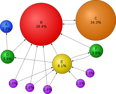
Motivation: PageRank

Source: Wikepedia
-
$\mathbf{A} \in {0,1}^{n \times n}$ the connectivity matrix of webpages with entries \(\begin{eqnarray*} a_{ij} = \begin{cases} 1 & \text{if page $i$ links to page $j$} \\ 0 & \text{otherwise} \end{cases}. \end{eqnarray*}\) $n \approx 10^9$ in May 2017.
-
$r_i = \sum_j a_{ij}$ is the out-degree of page $i$.
- Larry Page imagined a random surfer wandering on internet according to following rules:
- From a page $i$ with $r_i>0$
- with probability $p$, (s)he randomly chooses a link $j$ from page $i$ (uniformly) and follows that link to the next page
- with probability $1-p$, (s)he randomly chooses one page from the set of all $n$ pages (uniformly) and proceeds to that page
- From a page $i$ with $r_i=0$ (a dangling page), (s)he randomly chooses one page from the set of all $n$ pages (uniformly) and proceeds to that page
- From a page $i$ with $r_i>0$
-
The process defines an $n$-state Markov chain, where each state corresponds to each page. \(p_{ij} = (1-p)\frac{1}{n} + p\frac{a_{ij}}{r_i}\) with interpretation $a_{ij}/r_i = 1/n$ if $r_i = 0$.
-
Stationary distribution of this Markov chain gives the score (long term probability of visit) of each page.
-
Stationary distribution can be obtained as the top left eigenvector of the transition matrix $\mathbf{P}=(p_{ij})$ corresponding to eigenvalue 1. \(\mathbf{x}^T\mathbf{P} = \mathbf{x}^T.\) Equivalently it can be cast as a linear equation. \((\mathbf{I} - \mathbf{P}^T) \mathbf{x} = \mathbf{0}.\)
-
You’ve got to solve a linear equation with $10^9$ variables!
-
GE/LU will take $2 \times (10^9)^3/3/10^{12} \approx 6.66 \times 10^{14}$ seconds $\approx 20$ million years on a tera-flop supercomputer!
- Iterative methods come to the rescue.
Splitting and fixed point iteration
-
The key idea of iterative method for solving $\mathbf{A}\mathbf{x}=\mathbf{b}$ is to split the matrix $\mathbf{A}$ so that \(\mathbf{A} = \mathbf{M} - \mathbf{K}\) where $\mathbf{M}$ is invertible and easy to invert.
-
Then $\mathbf{A}\mathbf{x} = \mathbf{M}\mathbf{x} + \mathbf{K}\mathbf{x} = \mathbf{b}$ or \(\mathbf{x} = \mathbf{M}^{-1}\mathbf{K}\mathbf{x} + \mathbf{M}^{-1}\mathbf{b} .\) Thus a solution to $\mathbf{A}\mathbf{x}=\mathbf{b}$ is a fixed point of iteration \(\mathbf{x}^{(t+1)} = \mathbf{M}^{-1}\mathbf{K}\mathbf{x}^{(t)} + \mathbf{M}^{-1}\mathbf{b} = \mathbf{R}\mathbf{x}^{(k)} + \mathbf{c} .\)
-
Under a suitable choice of $\mathbf{R}$, i.e., splitting of $\mathbf{A}$, the sequence $\mathbf{x}^{(k)}$ generated by the above iteration converges to a solution $\mathbf{A}\mathbf{x}=\mathbf{b}$:
Let $\rho(\mathbf{R})=\max_{i=1,\dotsc,n} \lambda_i(\mathbf{R}) $, where $\lambda_i(\mathbf{R})$ is the $i$th (complex) eigenvalue of $\mathbf{R}$. When $\mathbf{A}$ is invertible, the iteration $\mathbf{x}^{(t+1)}=\mathbf{R}\mathbf{x}^{(t)} + \mathbf{c}$ converges to $\mathbf{A}^{-1}\mathbf{b}$ for any $\mathbf{x}^{(0)}$ if and only if $\rho(\mathbf{R}) < 1$.
Review of vector norms
A norm $|\cdot|: \mathbb{R}^n \to \mathbb{R}$ is defined by the following properties:
- $|\mathbf{x}| \ge 0$,
- $|\mathbf{x}| = 0 \iff \mathbf{x} = \mathbf{0}$,
-
$|c\mathbf{x}| = c |\mathbf{x}|$ for all $c \in \mathbb{R}$, - $|\mathbf{x} + \mathbf{y}| \le |\mathbf{x}| + |\mathbf{y}|$.
Typicall norms are
- $\ell_2$ (Euclidean) norm: $|\mathbf{x}| = \sqrt{\sum_{i=1}^nx_i^2}$;
-
$\ell_1$ norm: $|\mathbf{x}| = \sum_{i=1}^n x_i $; -
$\ell_{\infty}$ (Manhatan) norm: $|\mathbf{x}| = \max_{i=1,\dots,n} x_i $;
Matrix norms
- Matrix $\mathbf{A} \in \mathbb{R}^{n\times n}$ can be considered as a vector in $\mathbb{R}^{n^2}$.
- However, it is convinient if a matrix norm is compatible with matrix multiplication.
- In addition to the defining properties of a norm above, we require
- $|\mathbf{A}\mathbf{B}| \le |\mathbf{A}||\mathbf{A}|$.
Typical matrix norms are
- Frobenius norm: $|\mathbf{A}|F = \sqrt{\sum{i,j=1}^n a_{ij}^2} = \sqrt{\text{trace}(\mathbf{A}\mathbf{A}^T)}$;
- Operator norm (induced by a vector norm $|\cdot|$): $|\mathbf{A}| = \sup_{\mathbf{y}\neq\mathbf{0}}\frac{|\mathbf{A}\mathbf{y}|}{|\mathbf{y}|}$.
It can be shown that
-
$|\mathbf{A}|1 = \max{j=1,\dotsc,n}\sum_{i=1}^n a_{ij} $; -
$|\mathbf{A}|{\infty} = \max{i=1,\dotsc,n}\sum_{j=1}^n a_{ij} $; - $|\mathbf{A}|_2 = \sqrt{\rho(\mathbf{A}^T\mathbf{A})}$.
Convergence of iterative methods
- Let $\mathbf{x}^{\star}$ be a solution of $\mathbf{A}\mathbf{x} = \mathbf{b}$.
- Equivalently, $\mathbf{x}^{\star}$ satisfies $\mathbf{x}^{\star} = \mathbf{R}\mathbf{x}^{\star} + \mathbf{c}$.
- Subtracting this from $\mathbf{x}^{(t+1)} = \mathbf{R}\mathbf{x}^{(t)} + \mathbf{c}$, we have \(\mathbf{x}^{(t+1)} - \mathbf{x}^{\star} = \mathbf{R}(\mathbf{x}^{(t)} - \mathbf{x}^{\star}).\)
- Take a vector norm on both sides: \(\|\mathbf{x}^{(t+1)} - \mathbf{x}^{\star}\| = \|\mathbf{R}(\mathbf{x}^{(t)} - \mathbf{x}^{\star})\| \le \|\mathbf{R}\|\|\mathbf{x}^{(t)} - \mathbf{x}^{\star}\|\) where $|\mathbf{R}|$ is the induced operator norm.
- Thus if $|\mathbf{R}| < 1$ for a certain (induced) norm, then $\mathbf{x}^{(t)} \to \mathbf{x}^{\star}$.
Theorem. The spectral radius $\rho(\mathbf{A})$ of a matrix $\mathbf{A}\in\mathbb{R}^{n\times n}$ satisfies \(\rho(\mathbf{A}) \le \|\mathbf{A}\|\) for any operator norm. Furthermore, for any $\mathbf{A}\in\mathbb{R}^{n\times n}$ and $\epsilon > 0$, there is an operator norm $|\cdot|$ such that $|\mathbf{A}| \le \rho(\mathbf{A}) + \epsilon$.
Thus it is immediate to see \(\rho(\mathbf{A}) < 1 \iff \|\mathbf{A}\| < 1\) for some operator norm.
Proof. If $\lambda$ is an eigenvalue of $\mathbf{A}$ with nonzero eigenvector $\mathbf{v}$, then \(\|\mathbf{A}\mathbf{v}\| = |\lambda|\|\mathbf{v}\|\) (for a vector norm). So \(|\lambda| = \frac{\|\mathbf{A}\mathbf{v}\|}{\|\mathbf{v}\|} \le \|\mathbf{A}\|,\) implying the first inequality.
For the second part, suppose $\mathbf{A}\in\mathbb{R}^{n\times n}$ and $\epsilon > 0$ are given. Then there exist an (complex) upper triangular matrix $\mathbf{T}$ and an invertible matrix $\mathbf{S}$ such that \(\mathbf{A} = \mathbf{S}\mathbf{T}\mathbf{S}^{-1}\) and the eigenvalues of $\mathbf{A}$ coincides with the diagonal entries of $\mathbf{T}$. (Schur decomposition).
For $\delta > 0$ consider a diagonal matrix $\mathbf{D}(\delta)=\text{diag}(1, \delta, \delta^2, \dotsc, \delta^{n-1})$, which is invertible. Then
\[\mathbf{T}(\delta) \triangleq \mathbf{D}(\delta)^{-1}\mathbf{T}\mathbf{D}(\delta) =\mathbf{D}(\delta)^{-1}\mathbf{S}^{-1}\mathbf{A}\mathbf{S}\mathbf{D}(\delta) = (\mathbf{S}\mathbf{D}(\delta))^{-1}\mathbf{A}(\mathbf{S}\mathbf{D}(\delta))\]is an upper triangular matrix with entries $(\delta^{j-i}t_{ij})$ for $j \ge i$. So the off-diagonal entries tends to 0 as $\delta \to 0$.
Check \(\|\mathbf{x}\|_{\delta} := \|(\mathbf{S}\mathbf{D}(\delta))^{-1}\mathbf{x}\|_{\infty}\) defines a vector norm, which induces
\[\begin{split} \|\mathbf{A}\|_{\delta} &\triangleq \sup_{\mathbf{x}\neq\mathbf{0}}\frac{\|\mathbf{A}\mathbf{x}\|_{\delta}}{\|\mathbf{x}\|_{\delta}} = \sup_{\mathbf{x}\neq\mathbf{0}}\frac{\|[\mathbf{S}\mathbf{D}(\delta)]^{-1}\mathbf{A}\mathbf{x}\|_{\infty}}{\|[\mathbf{S}\mathbf{D}(\delta)]^{-1}\mathbf{x}\|_{\infty}} \\ &= \|(\mathbf{S}\mathbf{D}(\delta))^{-1}\mathbf{A}(\mathbf{S}\mathbf{D}(\delta))\|_{\infty} = \|\mathbf{T}(\delta)\|_{\infty} = \max_{i=1,\dotsc,n}\sum_{j=i}^n |t_{ij}|\delta^{j-i}. \end{split}\]Now since the eigenvalues of $\mathbf{A}$ coincides with $t_{ii}$, for each $\epsilon>0$ we can take a sufficiently small $\delta > 0$ so that \(\max_{i=1,\dotsc,n}\sum_{j=i}^n |t_{ij}|\delta^{j-i} \le \rho(\mathbf{A}) + \epsilon.\) This implies $|\mathbf{A}|_{\delta} \le \rho(\mathbf{A}) + \epsilon$.
- The only if part when $\mathbf{A}$ is inverible (hence $\mathbf{x}^{\star}$ is unique):
| If LHS converges to zero for any $\mathbf{x}^{(0)}$, then $\mathbf{R}^t \to \mathbf{0}$ as $t \to \infty$. This cannot occur if $ | \lambda_i(\mathbf{R}) | \ge 1$ for some $i$. |
Jacobi’s method
\[x_i^{(t+1)} = \frac{b_i - \sum_{j=1}^{i-1} a_{ij} x_j^{(t)} - \sum_{j=i+1}^n a_{ij} x_j^{(t)}}{a_{ii}}.\]-
Split $\mathbf{A} = \mathbf{L} + \mathbf{D} + \mathbf{U}$ = (strictly lower triangular) + (diagonal) + (strictly upper triangular).
-
Take $\mathbf{M}=\mathbf{D}$ (easy to invert!) and $\mathbf{K}=-(\mathbf{L} + \mathbf{U})$: \(\mathbf{D} \mathbf{x}^{(t+1)} = - (\mathbf{L} + \mathbf{U}) \mathbf{x}^{(t)} + \mathbf{b},\) i.e., \(\mathbf{x}^{(t+1)} = - \mathbf{D}^{-1} (\mathbf{L} + \mathbf{U}) \mathbf{x}^{(t)} + \mathbf{D}^{-1} \mathbf{b} = - \mathbf{D}^{-1} \mathbf{A} \mathbf{x}^{(t)} + \mathbf{x}^{(t)} + \mathbf{D}^{-1} \mathbf{b}.\)
-
Convergence is guaranteed if $\mathbf{A}$ is striclty row diagonally dominant: $ a_{ii} > \sum_{j\neq i} a_{ij} $. -
One round costs $2n^2$ flops with an unstructured $\mathbf{A}$. Gain over GE/LU if converges in $o(n)$ iterations.
- Saving is huge for sparse or structured $\mathbf{A}$. By structured, we mean the matrix-vector multiplication $\mathbf{A} \mathbf{v}$ is fast ($O(n)$ or $O(n \log n)$).
- Often the multiplication is implicit and $\mathbf{A}$ is not even stored, e.g., finite difference: $(\mathbf{A}\mathbf{v})i = v_i - v{i+1}$.
Gauss-Seidel method
\[x_i^{(t+1)} = \frac{b_i - \sum_{j=1}^{i-1} a_{ij} x_j^{(t+1)} - \sum_{j=i+1}^n a_{ij} x_j^{(t)}}{a_{ii}}.\]-
Split $\mathbf{A} = \mathbf{L} + \mathbf{D} + \mathbf{U}$ = (strictly lower triangular) + (diagonal) + (strictly upper triangular) as Jacobi.
-
Take $\mathbf{M}=\mathbf{D}+\mathbf{L}$ (easy to invert, why?) and $\mathbf{K}=-\mathbf{U}$: \((\mathbf{D} + \mathbf{L}) \mathbf{x}^{(t+1)} = - \mathbf{U} \mathbf{x}^{(t)} + \mathbf{b}\) i.e., \(\mathbf{x}^{(t+1)} = - (\mathbf{D} + \mathbf{L})^{-1} \mathbf{U} \mathbf{x}^{(t)} + (\mathbf{D} + \mathbf{L})^{-1} \mathbf{b}.\)
-
Equivalent to \(\mathbf{D}\mathbf{x}^{(t+1)} = - \mathbf{L} \mathbf{x}^{(t+1)} - \mathbf{U} \mathbf{x}^{(t)} + \mathbf{b}\) or \(\mathbf{x}^{(t+1)} = \mathbf{D}^{-1}(- \mathbf{L} \mathbf{x}^{(t+1)} - \mathbf{U} \mathbf{x}^{(t)} + \mathbf{b})\) leading to the iteration.
-
“Coordinate descent” version of Jacobi.
-
Convergence is guaranteed if $\mathbf{A}$ is striclty row diagonally dominant.
Successive over-relaxation (SOR)
\[x_i^{(t+1)} = \frac{\omega}{a_{ii}} \left( b_i - \sum_{j=1}^{i-1} a_{ij} x_j^{(t+1)} - \sum_{j=i+1}^n a_{ij} x_j^{(t)} \right)+ (1-\omega) x_i^{(t)},\]- $\omega=1$: Gauss-Seidel; $\omega \in (0, 1)$: underrelaxation; $\omega > 1$: overrelaxation
- Relaxation in hope of faster convergence
-
Split $\mathbf{A} = \mathbf{L} + \mathbf{D} + \mathbf{U}$ = (strictly lower triangular) + (diagonal) + (strictly upper triangular) as before.
- Take $\mathbf{M}=\frac{1}{\omega}\mathbf{D}+\mathbf{L}$ (easy to invert, why?) and $\mathbf{K}=\frac{1-\omega}{\omega}\mathbf{D}-\mathbf{U}$: \(\begin{split} (\mathbf{D} + \omega \mathbf{L})\mathbf{x}^{(t+1)} &= [(1-\omega) \mathbf{D} - \omega \mathbf{U}] \mathbf{x}^{(t)} + \omega \mathbf{b} \\ \mathbf{D}\mathbf{x}^{(t+1)} &= (1-\omega) \mathbf{D}\mathbf{x}^{(t)} + \omega ( -\mathbf{U}\mathbf{x}^{(t)} - \mathbf{L}\mathbf{x}^{(t+1)} + \mathbf{b} ) \\ \mathbf{x}^{(t+1)} &= (1-\omega)\mathbf{x}^{(t)} + \omega \mathbf{D}^{-1} ( -\mathbf{U}\mathbf{x}^{(t)} - \mathbf{L}\mathbf{x}^{(t+1)} + \mathbf{b} ) \end{split}\)
Conjugate gradient method
-
Conjugate gradient and its variants are the top-notch iterative methods for solving huge, structured linear systems.
-
Key idea: solving $\mathbf{A} \mathbf{x} = \mathbf{b}$ is equivalent to minimizing the quadratic function $\frac{1}{2} \mathbf{x}^T \mathbf{A} \mathbf{x} - \mathbf{b}^T \mathbf{x}$ if $\mathbf{A}$ is positive definite.
| Method | Number of Iterations |
|---|---|
| Gauss-Seidel | 208,000 |
| Block SOR methods | 765 |
| Incomplete Cholesky conjugate gradient | 25 |
- We defer the details of CG to the graduate-level Advanced Statistical Computing course.
Numerical examples
The Rlinsolve package implements most commonly used iterative solvers.
Generate test matrix
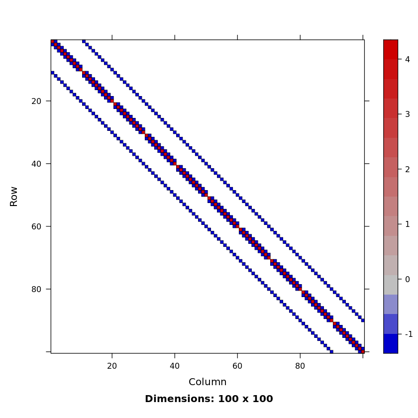
Poisson matrix is a block tridiagonal matrix from (discretized) Poisson’s equation $\nabla^2\psi = f$ in on the plane (with a certain boundary condition). This matrix is sparse, symmetric positive definite and has known eigenvalues.
Reference: G. H. Golub and C. F. Van Loan, Matrix Computations, second edition, Johns Hopkins University Press, Baltimore, Maryland, 1989 (Section 4.5.4).
get1DPoissonMatrix <- function(n) {
      Matrix::bandSparse(n, n, #dimensions
                        (-1):1, #band, diagonal is number 0
                        list(rep(-1, n-1),
                        rep(4, n),
                        rep(-1, n-1)))
}
get2DPoissonMatrix <- function(n) {  # n^n by n^n
    T <- get1DPoissonMatrix(n)
    eye <- Matrix::Diagonal(n)
    N <- n * n  ## dimension of the final square matrix
    ## construct two block diagonal matrices
    D <- bdiag(rep.int(list(T), n))
    O <- bdiag(rep.int(list(-eye), n - 1))

    ## augment O and add them together with D
    D +
     rbind(cbind(Matrix(0, nrow(O), n), O), Matrix(0, n, N)) +
     cbind(rbind(Matrix(0, n, ncol(O)), O), Matrix(0, N, n))
}
M <- get2DPoissonMatrix(10)
SparseM::image(M)

n <- 50
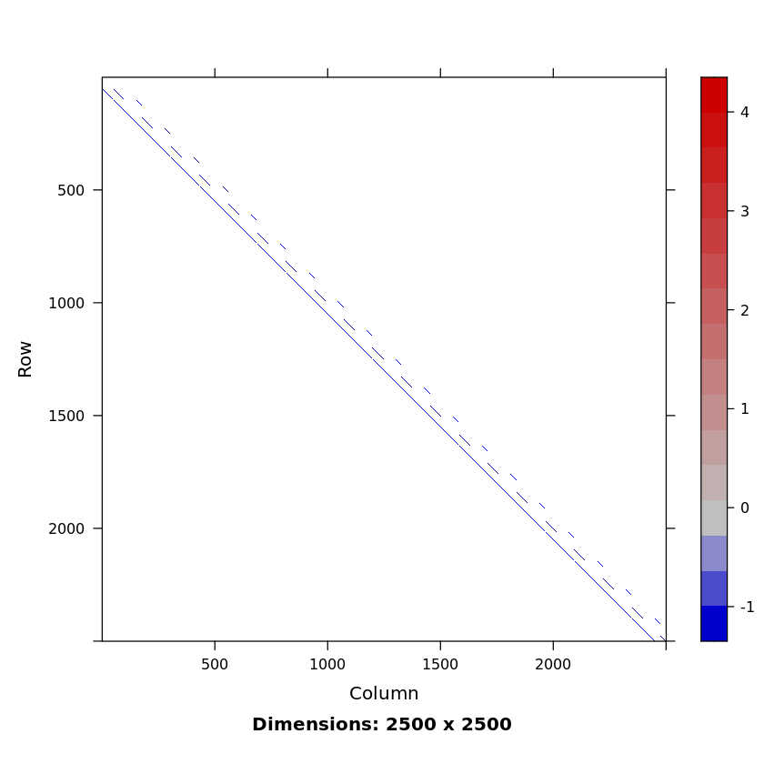
# Poisson matrix of dimension n^2=2500 by n^2, pd and sparse
A <- get2DPoissonMatrix(n)  # sparse
# dense matrix representation of A
Afull <- as.matrix(A)
# sparsity level
nnzero(A) / length(A)
0.001968
SparseM::image(A)

# storage difference
lobstr::obj_size(A)
lobstr::obj_size(Afull)
159,104 B


50,000,392 B
Matrix-vector muliplication
# randomly generated vector of length n^2
set.seed(123) # seed
b <- rnorm(n^2)
# dense matrix-vector multiplication
res <- microbenchmark::microbenchmark(Afull %*% b, A %*% b)
print(res)
Unit: microseconds
        expr       min        lq       mean     median         uq       max
 Afull %*% b 11717.114 12092.330 12443.1154 12225.3910 12389.8495 17404.718
     A %*% b    53.085    61.068   116.1806   124.4725   146.3725  1250.945
 neval cld
   100   b
   100  a
Dense solve via Cholesky
# record the Cholesky solution
#Achol <- base::chol(Afull)   # awfully slow
Achol <- Matrix::Cholesky(A)  # sparse Cholesky
# two triangular solves;  2n^2 flops
#y <- solve(t(Achol), b)
#xchol <- solve(Achol, y)
xchol <- solve(Achol, b)
Jacobi solver
It seems that Jacobi solver doesn’t give the correct answer.
xjacobi <- Rlinsolve::lsolve.jacobi(A, b)
Matrix::norm(xjacobi$x - xchol, 'F') / Matrix::norm(xchol, 'F')
* lsolve.jacobi : Initialiszed.

* lsolve.jacobi : computations finished.
0.139052743017417
Documentation reveals that the default value of maxiter is 1000. A couple trial runs shows that 5000 Jacobi iterations are required to get an “accurate enough” solution.
xjacobi <- Rlinsolve::lsolve.jacobi(A, b, maxiter=5000)
Matrix::norm(xjacobi$x - xchol, 'F') / Matrix::norm(xchol, 'F')
* lsolve.jacobi : Initialiszed.

* lsolve.jacobi : computations finished.
0.00194359601984354
xjacobi$iter
4345
Gauss-Seidel
# Gauss-Seidel solution is fairly close to Cholesky solution after 5000 iters
xgs <- Rlinsolve::lsolve.gs(A, b, maxiter=5000)
Matrix::norm(xgs$x - xchol, 'F') / Matrix::norm(xchol, 'F')
* lsolve.gs : Initialiszed.

* lsolve.gs : computations finished.
0.00194122159891645
xgs$iter
1425
SOR
# symmetric SOR with ω=0.75
xsor <- Rlinsolve::lsolve.ssor(A, b, w=0.75, maxiter=5000)
Matrix::norm(xsor$x - xchol, 'F') / Matrix::norm(xchol, 'F')
* lsolve.ssor : Initialiszed.

* lsolve.ssor : computations finished.
0.0019608277003874
xsor$iter
1204
Conjugate Gradient
# conjugate gradient
xcg <- Rlinsolve::lsolve.cg(A, b)
Matrix::norm(xcg$x - xchol, 'F') / Matrix::norm(xchol, 'F')
* lsolve.cg : Initialiszed.

* lsolve.cg : preprocessing finished ...

* lsolve.cg : convergence was well achieved.

* lsolve.cg : computations finished.
1.3334483963847e-05
xcg$iter
113
- A basic tenet in numerical analysis:
The structure should be exploited whenever possible in solving a problem.

Comments