40 min to read
[통계계산] 9. Random Number Generation
Computational Statistics

[통계계산] 9. Numerical Integration
목차
- Computer Arithmetic
- LU decomposition
- Cholesky Decomposition
- QR Decomposition
- Interative Methods
- Non-linear Equations
- Optimization
- Numerical Integration
- Random Number Generation
- Monte Carlo Integration
sessionInfo()
R version 3.6.3 (2020-02-29)
Platform: x86_64-pc-linux-gnu (64-bit)
Running under: Ubuntu 18.04.5 LTS

Matrix products: default
BLAS:   /usr/lib/x86_64-linux-gnu/blas/libblas.so.3.7.1
LAPACK: /usr/lib/x86_64-linux-gnu/lapack/liblapack.so.3.7.1

locale:
 [1] LC_CTYPE=en_US.UTF-8       LC_NUMERIC=C
 [3] LC_TIME=en_US.UTF-8        LC_COLLATE=en_US.UTF-8
 [5] LC_MONETARY=en_US.UTF-8    LC_MESSAGES=en_US.UTF-8
 [7] LC_PAPER=en_US.UTF-8       LC_NAME=C
 [9] LC_ADDRESS=C               LC_TELEPHONE=C
[11] LC_MEASUREMENT=en_US.UTF-8 LC_IDENTIFICATION=C

attached base packages:
[1] stats     graphics  grDevices utils     datasets  methods   base

other attached packages:
[1] scatterplot3d_0.3-41

loaded via a namespace (and not attached):
 [1] fansi_0.5.0       digest_0.6.27     utf8_1.2.1        crayon_1.4.1
 [5] IRdisplay_1.0     repr_1.1.3        lifecycle_1.0.0   jsonlite_1.7.2
 [9] evaluate_0.14     pillar_1.6.1      rlang_0.4.11      uuid_0.1-4
[13] vctrs_0.3.8       ellipsis_0.3.2    IRkernel_1.1      tools_3.6.3
[17] compiler_3.6.3    base64enc_0.1-3   pbdZMQ_0.3-5      htmltools_0.5.1.1
# install.packages("ggplot2")

library(scatterplot3d)
library(ggplot2)
Registered S3 methods overwritten by 'tibble':
  method     from
  format.tbl pillar
  print.tbl  pillar

Registered S3 methods overwritten by 'ggplot2':
  method         from
  [.quosures     rlang
  c.quosures     rlang
  print.quosures rlang
Random number generation
Uniform random number generation
Goal
To generate $U_i \stackrel{iid}{\sim} \text{unif}(0, 1)$.
- Basis for all other random number generation
- Fact: NO RANDOM NUMBER IN COMPUTER — only look random (PSEUDO-RANDOM)
Congruential generator
\begin{align}
x_{i+1} &= a x_i \mod m, \quad i=1, 2, \dotsc
u_i &= x_i / m.
\end{align}
- Modulus $m$ is a large prime number.
- Multiplier $a$ is a positive integer between 2 and $m-1$.
- Map $f: x \mapsto ax \mod m$ maps ${1, \dotsc, m-1}$ onto itself and is one-to-one:
- Suppose $x\in{1, \dotsc, m-1}$. Then $f(x) \neq 0$ since $a$ and $m$ are relatively prime hence $ax$ is not a multiple of $m$. Thus $f$ maps ${1, , \dotsc, m-1}$ to ${1, , \dotsc, m-1}$.
- If $ay = ax \mod m$, then $a(y - x) = m k$ for some integer $k$. Since $a$ and $m$ are relatively prime, $y - x = m l$ for some interger $l$. That is, $x = y \mod m$. Hence map $f$ is one-to-one.
- Since $f$ maps ${1, , \dotsc, m-1}$ to ${1, , \dotsc, m-1}$ and one-to-one, $f$ is also onto.
- Note
\begin{align}
x_1 &= a x_0 \mod m
x_2 &= a x_1 \mod m = a^2 x_0 \mod m
x_3 &= a x_2 \mod m = a^3 x_0 \mod m
& \vdots
x_n &= a x_{n-1} \mod m = a^n x_0 \mod m \end{align} Hence if $a^n = 1 \mod m$ for some $n$, then \(x_n = x_0 \mod m\) and the (pseudo)random number generator repeats the sequence. The number $n$ is called the period of the RNG, and $x_0$ is called the seed.
set.seed(2020)  # set 2020th seed; does not mean x_0 = 2020
runif(5)
set.seed(2020)  # same seed results in same "random" sequence
runif(5)
<ol class=list-inline><li>0.646902838954702</li><li>0.394225758267567</li><li>0.618501814315096</li><li>0.476891135564074</li><li>0.136097185546532</li></ol>
<ol class=list-inline><li>0.646902838954702</li><li>0.394225758267567</li><li>0.618501814315096</li><li>0.476891135564074</li><li>0.136097185546532</li></ol>
- Primitive root of unity
- Fermat’s little theorem: $a^{m} = a \mod m$.
- Since $a$ is not divisible by $m$, we have $a^{m-1} = 1 \mod m$.
- Thus the period $n$ satisfies $n \le m - 1$.
- Primitive root of unity: $a$ such that $n = m - 1$
- If $a$ is primitive, then $x_1, x_2, \dotsc, x_{m-1}$ is a permutation of ${1, 2, \dotsc, m-1}$.
- For $m=2^{31} - 1$ (Mersenne prime), $a=7^5 = 16807$ is primitive, leading to the period of $2^{31} - 2$ =
2,147,483,646. This RNG was used in early versions of MATLAB (up to v4).
Good RNGs should have long periods, and should give samples which appear to be drawn from a uniform distribution. If the size of the sample is much less than the period of the RNG, then the sample should appear random.
Autocorrelation
-
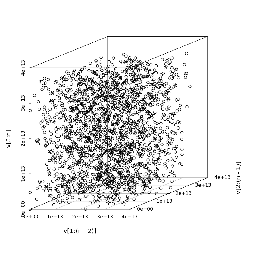
Ideally, a pseudorandom number sequence should look i.i.d. If we take the first $p$ values to form an $p$-dimensional vector, the second $p$ values to form a second $p$-dimensional vector, etc, then these vectors should fill the $p$-dimensional hypercube uniformly.
-
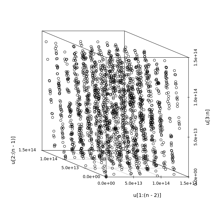
However, by construction the sequence generated by congruential generators depends on the previous value, hence tends to be correlated.
-
It is known that congruential generators tend to give $p$-dimensional vectors that concentrate lower-dimensional hyperplanes, for some $p$.
# IBM System/360 RANDU generator
# a = 2^16 + 3 = 65539
# m = 2^31
n <- 2000
a <- 65539
m <- 2^31
u <- vector(length=n)
u[1] <- 1
for (i in seq_len(n-1)) {
    u[i+1] <- a * u[i] %% m
}
scatterplot3d(u[1:(n-2)], u[2:(n-1)], u[3:n], angle=160)
# Early MATLAB RNG
# a = 7^5
# m = 2^31 - 1
n <- 2000
a2 <- 7^5
m2 <- 2^31 - 1
v <- vector(length=n)
v[1] <- 1
for (i in seq_len(n-1)) {
    v[i+1] <- a2 * v[i] %% m2
}
scatterplot3d(v[1:(n-2)], v[2:(n-1)], v[3:n], angle=20)
A simple modification is to introduce shuffling in the sequence, which we won’t cover in detail.
R’s RNG
-
R uses the Mersenne-Twister as the default RNG. This RNG was developed by Matsumoto and Nishimura in 1998, and is the first algorithm whose period ($2^{19937} - 1$) exceeds the number of electron spin changes since the creation of the Universe ($10^{6000}$ against $10^{120}$)!
-
Mersenne-Twister guarantees 623 consecutive dimensions to be equidistributed (over the whole period).
RNGkind()
<ol class=list-inline><li>‘Mersenne-Twister’</li><li>‘Inversion’</li><li>‘Rejection’</li></ol>
Transformation methods
From now on, we assume the the problem of generating uniform random numbers has been solved for practical purposes.
Inverse CDF method
For a random variable $X$, let $F$ be its cumulative distribution function (CDF), that is, $F(x) = P(X \le x)$. Recall that $F$ is right-continuous and nondecreasing. Also, if $F$ is strictrly increasing, random variable $F(X)$ is uniformly distributed on $[0, 1]$. Below, we generalize this result.
The inverse CDF of $X$ is defined as \(F^{-1}(u) = \inf\{x: F(x) \ge u\}, ,\) which coincides the usual inverse of $F$ if $F$ is strictly increasing.
Proposition 1. Let $X$ be a random variable with CDF $F$. Then the following holds.
- If $F$ is continuous, then $U = F(X)$ is a uniform random variable on $[0, 1]$.
- If $F$ is not continous, then $P[F(X) \le y] \le y$ for all $y \in [0, 1]$.
- If $U$ is uniform on $[0, 1]$, then $F^{-1}(U)$ has CDF $F$.
Proof.
- Part 1: We will show that \(P[F(X) \le F(t)] = F(t) \tag{*}\) for any $t$. Suppose for now this is true.
Let $u \in (0, 1)$. Then by continuity of $F$, there is $y$ such that $F(y) = u$. By (*), \(P[F(X) \le u] = P[F(X) \le F(y)] = F(y) = u.\)
-
Part 3: It suffices to show that ${F^{-1}(U) \le t} = {U \le F(t)}$. If $F^{-1}(u)=\inf{x: F(x) \ge u} \le t$, then by the monotonicity and right-continuity of $F$, the set ${x: F(x) \ge u}$ is an half-closed interval containing its left endpoint, which is $F^{-1}(u)$. Hence $F(F^{-1}(u)) \ge u$. Since $F^{-1}(u) \le t$, again by monotonicity of $F$, it follows that $u \le F(F^{-1}(u)) \le F(t)$. Conversely, if $u \le F(t)$, then by definition $F^{-1}(u) \le t$.
-
Part 2: by part 3, $X\stackrel{d}{=}F^{-1}(U)$, where $U$ is uniform on $[0, 1]$. Since $x=F^{-1}(u)$ implies $u \le F(x)$, \(P[F(X) \le y] \le P(U \le y) = y.\)
-
It remains to show (). Monotonicity of $F$ yields ${X > t} \subset {F(X) \ge F(t)}$. Hence ${X > t } \cap {F(X) < F(t) } = \emptyset$. Likewise ${X \le t} \cap {F(X) > F(t)} = \emptyset}$. Then, \begin{align} {X > t} \cap {F(X) \le F(t)} &= [{X > t} \cap {F(X) < F(t) }] \cup [{X > t} \cap {F(X) = F(t)}]
&= {X > t} \cap {F(X) = F(t)}
{X \le t} \cap {F(X) \le F(t)} &= {X \le t} \cap {F(X) > F(t)}^c = {X \le t} \end{align*} So, \(\{F(X) \le F(t) \} = \{X \le t\} \cup [\{X > t\} \cap \{F(X) = F(t)\}] =: A \cup B .\) Obviously events $A$ and $B$ are disjoint. However, event $B$ corresponds to the values $x$ of $X$ with which $F(x)$ is constant. Hence $P(B)=0$. Therefore, \(P[F(X) \le F(t)] = P(A) + P(B) = P(A) = P(X \le t) = F(t).\)
Exponential distribution
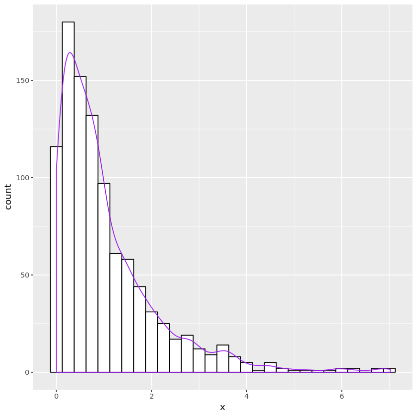
- CDF $F(x) = 1 - e^{-\lambda x}$ yields $F^{-1}(u) = -\frac{1}{\lambda}\log u$ on $(0, 1)$.
# Exp(1)
n <- 1000
u <- runif(n)
x <- -log(u)
expdata <- data.frame(x)
plt <- ggplot(expdata, aes(x=x)) +
    geom_histogram(binwidth=0.25, fill="white", color="black") +
    geom_density(aes(y=0.25 * ..count..), color="purple")
print(plt)
Cauchy distribution
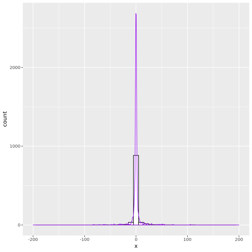
From the density of the Cauchy distribution \(f(x) = \frac{\beta}{\pi(\beta^2 + (x-\mu)^2)},\) its CDF is $F(x) = \frac{1}{2} + \frac{1}{\pi}\tan^{-1}\left(\frac{x-\mu}{\beta}\right)$. Thus \(F^{-1}(u) = \mu + \beta\tan(\pi u - \pi/2) = \mu - \frac{\beta}{\tan(\pi u)} .\)
# standard Cauchy (beta=1, mu=0)
n <- 1000
u <- runif(n)
x <- -1/tan(pi * u)
#hist(x, breaks=40)
cauchydata <- data.frame(x)
plt <- ggplot(cauchydata, aes(x=x)) +
    geom_histogram(binwidth=10, fill="white", color="black") +
    geom_density(aes(y=10 * ..count..), color="purple") +
    xlim(-200, 200)
print(plt)
Warning message:
“Removed 4 rows containing non-finite values (stat_bin).”
Warning message:
“Removed 4 rows containing non-finite values (stat_density).”
Warning message:
“Removed 2 rows containing missing values (geom_bar).”
Discrete uniform distribution
$X \sim \text{unif}({1, 2, \dotsc, k})$. It is easy to verify $F(x) = \frac{1}{k}\lfloor x \rfloor$ for $x \in [0, n]$ and $F^{-1}(u)=\lceil ku \rceil$.
k <- 10
n <- 1000
u <- runif(n)
x <- ceiling(k * u)
table(x)
x
  1   2   3   4   5   6   7   8   9  10
108 108  92  93  97  85  94 118 108  97
Geometric distribution
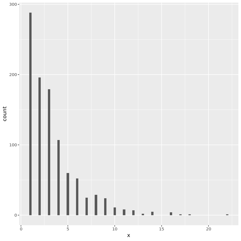
If $X \sim \text{geom}(p)$, then its probability mass functin $p(x) = (1-p)^{x-1}p$.
For $Y \sim \text{Exp}(\lambda)$,
\begin{align}
P(\lceil Y \rceil = k) &= P(k-1 < Y \le k) = F_Y(k) - F_Y(k-1) = (1 - e^{-\lambda k}) - (1 - e^{-\lambda(k-1)})
&= e^{-\lambda(k-1)}(1 - e^{-\lambda})
&- (1 - p)^{k-1} p
\end{align}
if $\lambda$ satisfies $p = 1 - e^{-\lambda}$, or $\lambda = -\log(1-p)$.
For this $\lambda$, $X = \lceil Y \rceil = \lceil -\frac{1}{\lambda}\log U \rceil = \lceil \frac{\log U}{\log(1-p)}\rceil$.
gengeom <- function(p, nsamp=1) {
    u <- runif(nsamp)
    y <- log(u) / log(1 - p)
    ceiling(y)
}
nsamp <- 1000
p <- 0.3
x <- gengeom(p, nsamp)
geomdata <- data.frame(x)
plt <- ggplot(geomdata, aes(x=x)) + geom_histogram(binwidth=0.25)
print(plt)
Normal random numbers
For $X \sim N(0, 1)$, inverse CDF $\Phi^{-1}$ does not have a closed form.
Box-Muller
Generates $X, Y \stackrel{iid}{\sim} N(0, 1)$.
Transforms the random Cartesian coordinates $(X, Y)$ to polar coorinates $(R, \Theta)$. Since $(X, Y)=(R\cos\Theta, R\sin\Theta)$, \(\iint f_{XY}(x, y)dxdy = \frac{1}{2\pi}\exp(-\frac{x^2 + y^2}{2})dxdy = \iint \frac{1}{2\pi}\exp(-\frac{r^2}{2})rdrd\theta .\)
Hence $R$ has density $f_R(r) = r\exp(-\frac{r^2}{2})$ and $\Theta$ is uninform on $[0, 2\pi]$. Since \(P(R > \rho) = P(R^2 > \rho^2) = \int_\rho^{\infty} r\exp(-\frac{r^2}{2})dr = \exp(-\frac{1}{2}\rho^2),\) random variable $R^2$ is exponentially distributed with $\lambda = 1/2$.
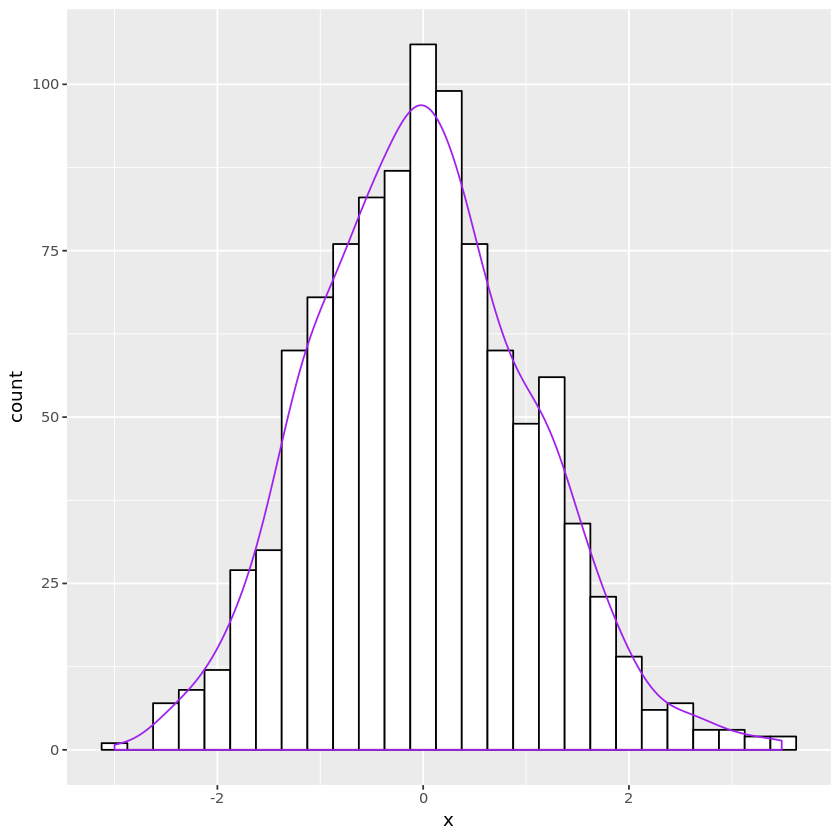
Thus for independent $U, V \sim \text{unif}(0, 1)$, set \(R = (-2\log U)^{1/2}, \quad \Theta = 2\pi V .\) Then $(X, Y) = (R\cos\Theta, R\sin\Theta)$ are independently $N(0, 1)$.
boxmuller <- function(nsamp) {
    n <- ceiling(nsamp / 2)
    u <- runif(n)
    v <- runif(n)
    r <- sqrt(-2 * log(u))
    theta <- 2 * pi * v
    x <- r * cos(theta)
    y <- r * sin(theta)
    samp <- c(x, y)
    samp[seq_len(nsamp)]
}
#hist(c(x, y))
n <- 1000
normdata1 <- data.frame(x = boxmuller(n))
plt <- ggplot(normdata1, aes(x=x)) +
    geom_histogram(binwidth=0.25, fill="white", color="black") +
    geom_density(aes(y=0.25 * ..count..), color="purple")
print(plt)
Marsaglia
-
From the Box-Muller transformation, we learned that if $R^2 \sim \text{Exp}(1/2)$ and $\Theta\sim\text{unif}(0, 2\pi)$ and they are independent, $(R\cos\Theta, R\sin\Theta)$ are i.i.d. standard normal.
-
On the other hand, if a random point $(U, V)$ is uniformly distributed on the unit disk, and let $(U, V) = (T\cos\Phi, T\sin\Phi)$, then \(P(T^2 \le t^2, 0 \le \Phi \le \phi) = \frac{t^2\phi}{2\pi}, \quad t^2 \le 1, ~ \phi \in (0, 2\pi) \\\) which means that $T^2 = U^2 + V^2 \sim \text{unif}(0, 1)$, $\Phi \sim \text{unif}(0, 2\pi)$, and they are independent.
-
Therefore, if we sample $(U, V)$ uniformly from the unit disk, and set $T = \sqrt{U^2 + V^2}$, $\cos\Phi = U/T$, $\sin\Phi=V/T$, then $T^2\sim\text{unif}(0,1)$ and $-2\log T^2$ is identically distributed to $R^2$, i.e., $\text{Exp}(1/2)$, and $\Phi$ is identically distributed to $\Theta$, i.e., uniform on $(0, 2\pi)$. Therefore, if we set $(X, Y)$ such that \(X = \sqrt{-2\log T^2}\frac{U}{T}, \quad Y = \sqrt{-2\log T^2}\frac{V}{T},\) then $X, Y$ are i.i.d. standard normal.
-
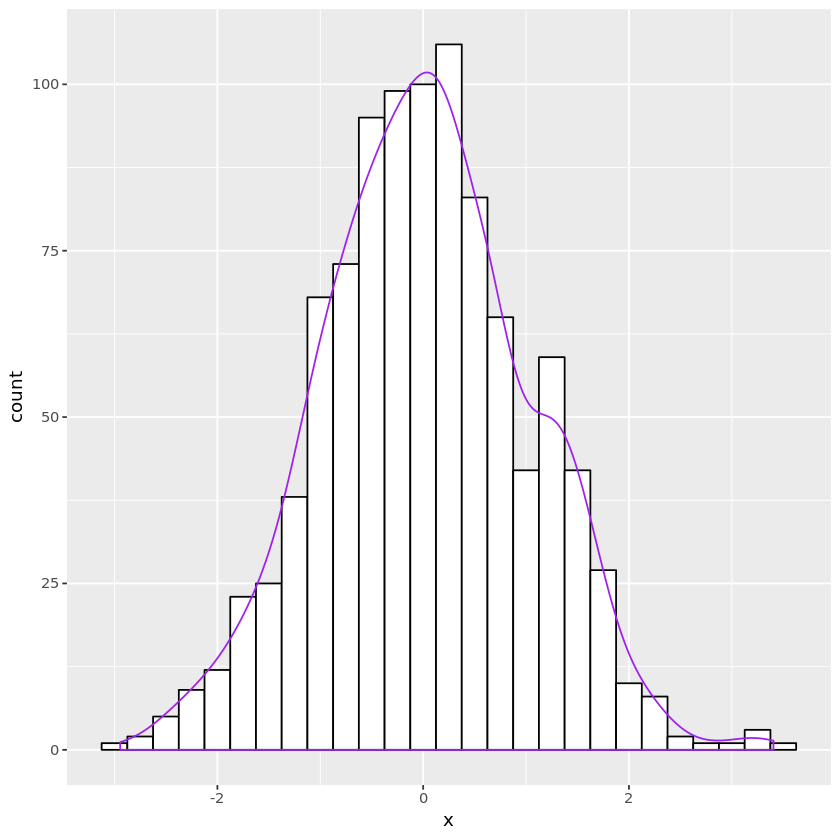
One way to sample from the unit disk is to sample $(U, V)$ from $\text{unif}[-1, 1]\times\text{unif}[-1, 1]$, and discard the sample if $U^2 + V^2 > 1$ and resample (see acceptance-rejection sampling below).
- Algorithm:
- $U, V \stackrel{iid}{\sim} \text{unif}[-1, 1]$;
- If $T = \sqrt{U^2 + V^2} > 1$, go to 1;
- Set $X = \sqrt{-2\log T^2}\frac{U}{T}$ and $Y = \sqrt{-2\log T^2}\frac{V}{T}$.
- This method avoids the trigonometric function evaluations of the Box-Muller, but uses $4/\pi$ as many random pairs on average.
marsaglia <- function(nsamp) {
    n <- ceiling(nsamp / 2)
    it <- 0
    x <- numeric(n)
    y <- numeric(n)
    while (it < n) {
        u <- 2 * runif(1) - 1
        v <- 2 * runif(1) - 1
        tau <- sqrt(u^2 + v^2)
        if (tau > 1) next
        x[it] <- sqrt(-4 * log(tau)) * u / tau
        y[it] <- sqrt(-4 * log(tau)) * v / tau
        it <- it + 1
    }
    samp <- c(x, y)
    samp[seq_len(nsamp)]
}
n <- 1000
normdata2 <- data.frame(x = marsaglia(n))
plt <- ggplot(normdata2, aes(x=x)) +
    geom_histogram(binwidth=0.25, fill="white", color="black") +
    geom_density(aes(y=0.25 * ..count..), color="purple")
print(plt)
Random numbers by definition
Bernoulli
- Set the success probability $p$
- Generate $U \sim \text{unif}(0, 1)$.
- Let $X = \mathbb{I}_{{U \le p}}$.
- Then $X \sim \text{Ber}(p)$.
Binomial
- Set the success probability $p$
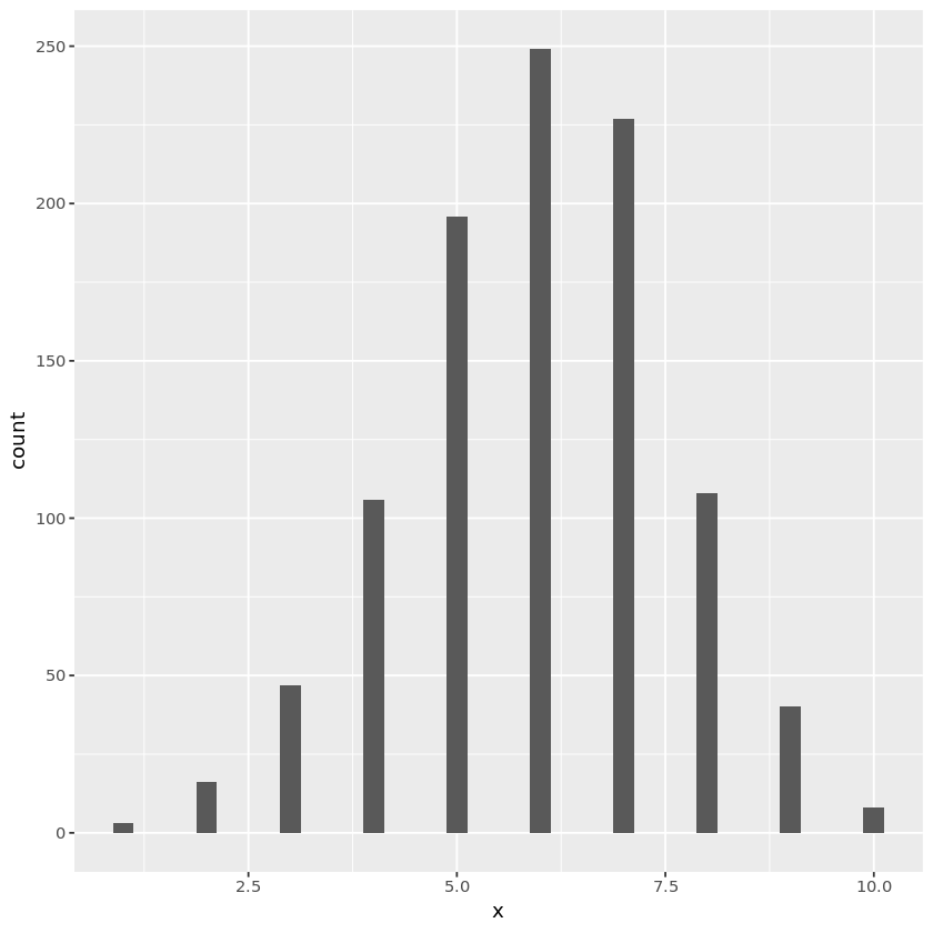
- Generate $n$ independent $X_i \sim \text{Ber}(p)$.
- Let $X_n = \sum_{i=1}^n X_i$.
- Then $X_n \sim B(n, p)$.
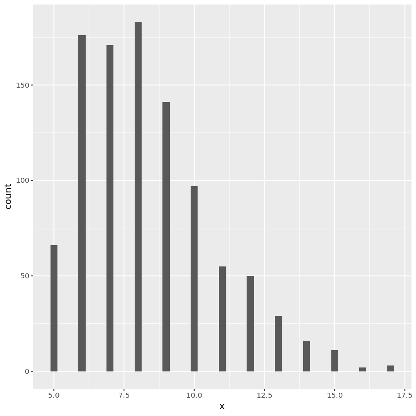
Negative binomial
- Set the success probability $p$
- Generate $r$ independent $X_i \sim \text{Geom}(p)$.
- Let $X_r = \sum_{i=1}^r X_i$.
- Then $X_r \sim \text{NegBin}(r, p)$.
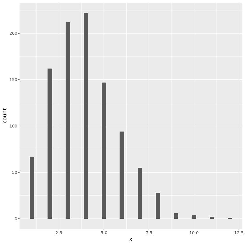
Poisson
- Generate $U_i \stackrel{iid}{\sim} \text{unif}(0, 1)$.
- Find $N$ such that $\prod_{i=1}^N U_i \ge e^{-\lambda} > \prod_{i=1}^{N+1} U_i$.
- Then $N \sim \text{Poi}(\lambda)$.
- This is because $T_i = -\frac{1}{\lambda}\log U_i \stackrel{iid}{\sim} \text{Exp}(\lambda)$, and is the waiting time between the $i-1$st and the $i$th event of the Poisson counting process $N(t) \sim \text{Poi}(\lambda t)$.
- That is, $N \sim \text{Poi}(\lambda) \iff T_1 + \dotsc + T_N \le 1 < T_1 + \dotsc + T_N + T_{N+1}$.
## Binomial random number generation
genbin <- function(n, p) {
    u <- runif(n)
    x <- sum(u < p)
}
n <- 10; p <- 0.6
nsamp <- 1000
x <- numeric(nsamp)
for (i in seq_len(nsamp)) {
    x[i] <- genbin(n, p)
}
bindata <- data.frame(x)
plt <- ggplot(bindata, aes(x=x)) + geom_histogram(binwidth=0.25)
print(plt)
# Negative binomial random number generation
gengeom <- function(p, nsamp=1) {
    u <- runif(nsamp)
    y <- log(u) / log(1 - p)
    ceiling(y)
}
nsamp <- 1000
p <- 0.6
r <- 5
x <- numeric(nsamp)
for (i in seq_len(r)) {
    x <- x + gengeom(p, nsamp)
}
negbindata <- data.frame(x)
plt <- ggplot(negbindata, aes(x=x)) + geom_histogram(binwidth=0.25)
print(plt)
# Poisson random number generation
genpoi <- function(lam, maxiter=1000) {
    u_cum <- 1.0
    k <- 0
    while (u_cum > exp(-lam) && k < maxiter ) {
        u <- runif(1)
        u_cum <- u_cum * u
        k <- k + 1
    }
    k
}
lam <- 3  # Poisson rate
nsamp <- 1000
x <- numeric(nsamp)
for (i in seq_len(nsamp)) {
    x[i] <- genpoi(lam)
}
poidata <- data.frame(x)
plt <- ggplot(poidata, aes(x=x)) + geom_histogram(binwidth=0.25)
print(plt)
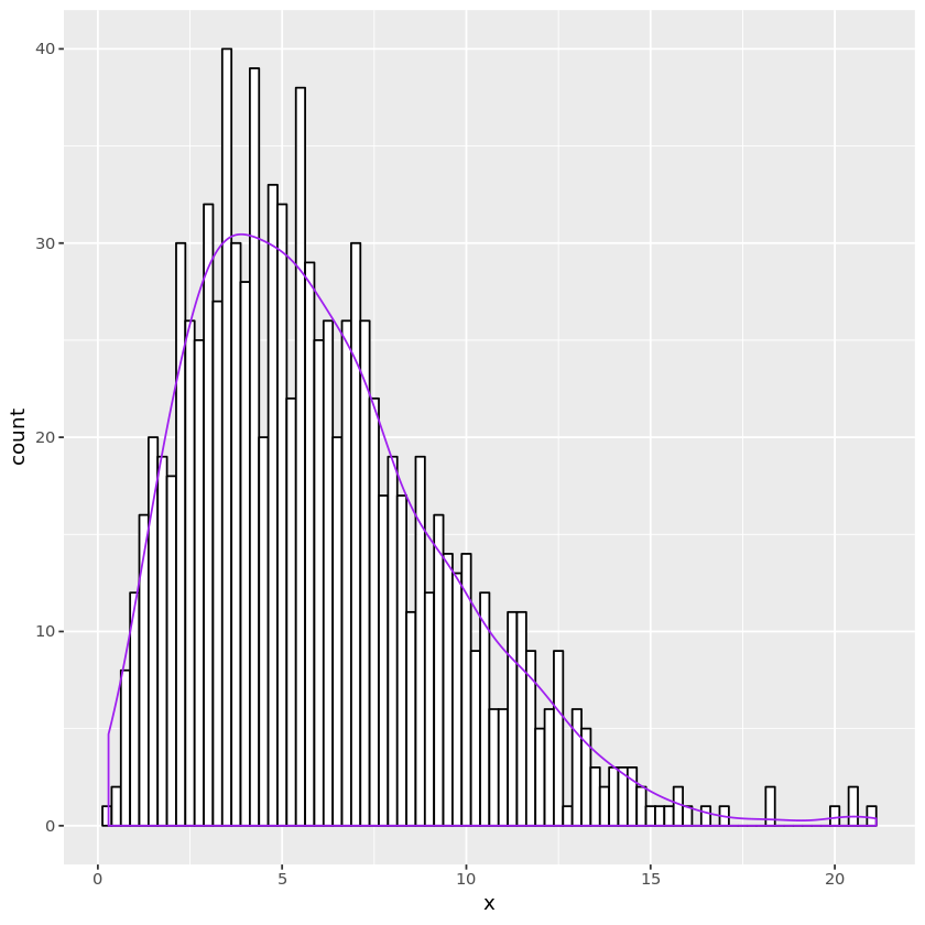
Chi-square
- Generate $Z_1, \dotsc, Z_{\nu} \stackrel{iid}{\sim} N(0, 1)$.
- Let $X_{\nu} = \sum_{i=1}^{\nu} Z_i^2$.
- Then $X_{\nu} \sim \chi^2(\nu)$.
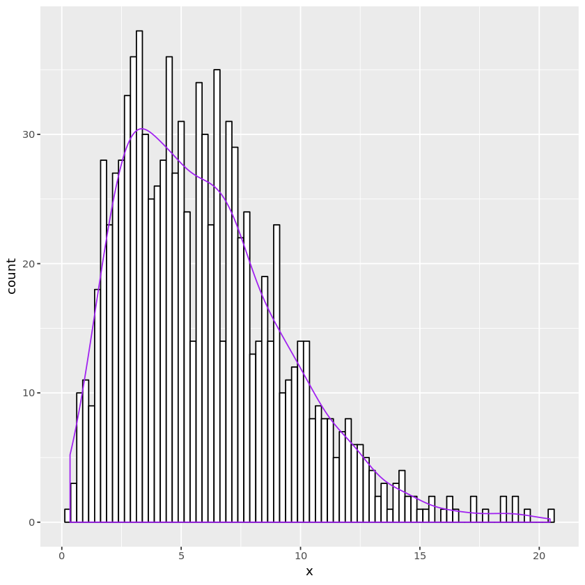
Alternatively, for even $\nu$:
- Generate $U_i \stackrel{iid}{\sim} \text{unif}(0, 1)$.
- Let $X_{\nu} = -2\log(\prod_{i=1}^{\nu/2} U_i)$.
- Then $X_{\nu} \sim \chi^2(\nu)$.
This is because $\chi^2(\nu) = \text{Gamma}(\nu/2, 2)$, where 2 is the scale parameter.
Student’s $t$
- Generate $Z \sim N(0, 1)$ and $X \sim \chi^2(\nu)$ independently.
- Let $T = Z / \sqrt{X/\nu}$.
- Then $T \sim t(\nu)$.
$F$
- Generate $X_1 \sim \chi^2(\nu_1)$ and $X_2 \sim \chi^2(\nu_2)$ independently.
- Let \(F = \frac{X_1/\nu_1}{X_2/\nu_2}.\)
- The $F \sim F(\nu_1, \nu_2)$.
## chi-square random number generation
genchisq1 <- function(nsamp, nu) {
    z <- matrix(rnorm(nsamp * nu), nrow=nsamp)
    rowSums(z^2)
}
nu <- 6
n <- 1000
chisqdata1 <- data.frame(x = genchisq1(n, nu))
plt <- ggplot(chisqdata1, aes(x=x)) +
    geom_histogram(binwidth=0.25, fill="white", color="black") +
    geom_density(aes(y=0.25 * ..count..), color="purple")
print(plt)
## chi-square random number generation 2
genchisq2 <- function(nsamp, nu) {
    u <- matrix(runif(nsamp * nu / 2), nrow=nsamp)
    -2 * log(apply(u, 1, prod) )
}
nu <- 6
n <- 1000
chisqdata2 <- data.frame(x = genchisq2(n, nu))
plt <- ggplot(chisqdata2, aes(x=x)) +
    geom_histogram(binwidth=0.25, fill="white", color="black") +
    geom_density(aes(y=0.25 * ..count..), color="purple")
print(plt)
## Student's t random number generation
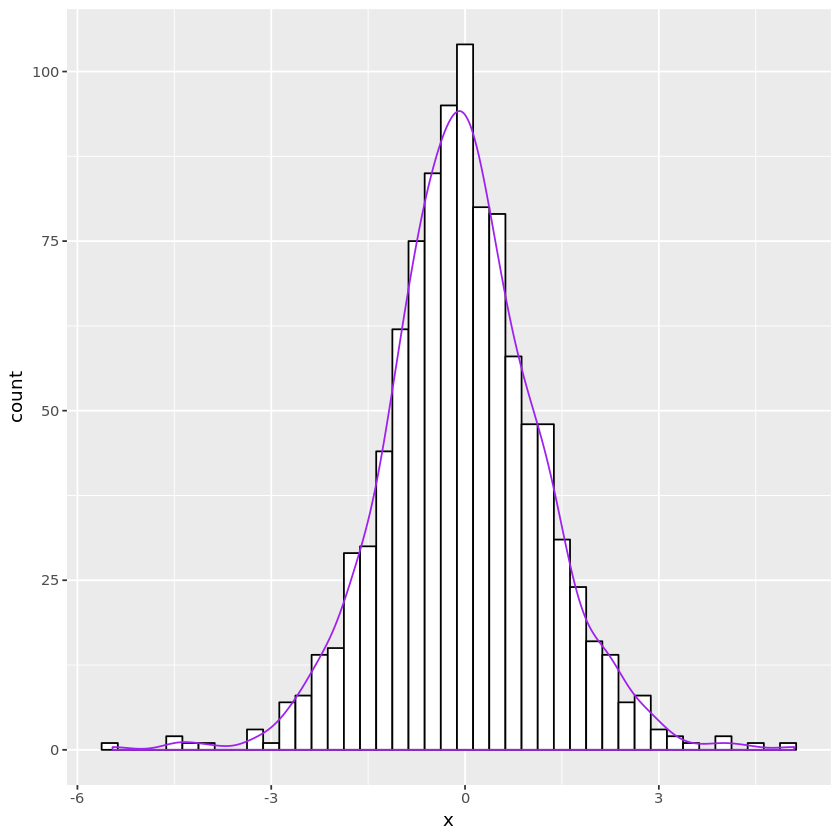
gent <- function(nsamp, nu) {
    z <- rnorm(nsamp)
    chisq <- genchisq1(nsamp, nu)
    trv <- z / sqrt(chisq / nu)
}
nu <- 6
n <- 1000
tdata <- data.frame(x = gent(n, nu))
plt <- ggplot(tdata, aes(x=x)) +
    geom_histogram(binwidth=0.25, fill="white", color="black") +
    geom_density(aes(y=0.25 * ..count..), color="purple")
print(plt)
# F random number generation
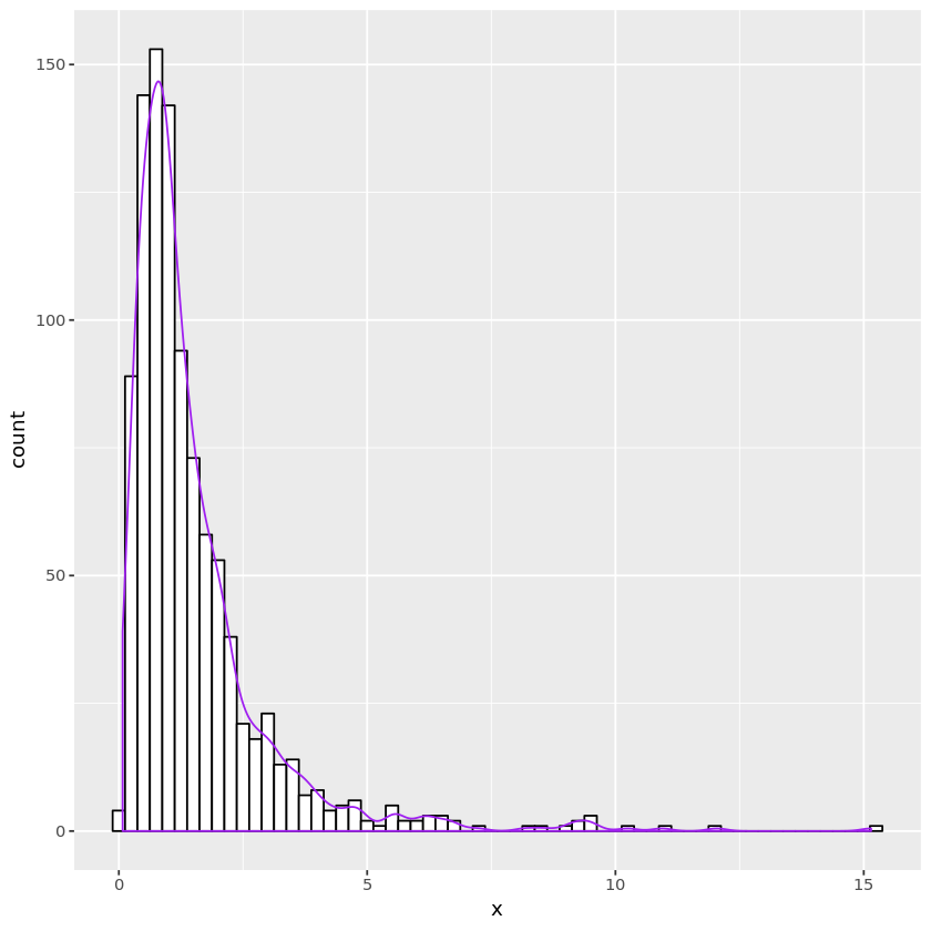
genF <- function(nsamp, nu1, nu2) {
    chisq1 <- genchisq1(nsamp, nu1)
    chisq2 <- genchisq1(nsamp, nu2)
    Frv <- chisq1 / nu1 / chisq2 * nu2
}
nu1 <- 10; nu2 <- 6
n <- 1000
Fdata <- data.frame(x = genF(n, nu1, nu2))
plt <- ggplot(Fdata, aes(x=x)) +
    geom_histogram(binwidth=0.25, fill="white", color="black") +
    geom_density(aes(y=0.25 * ..count..), color="purple")
print(plt)
Acceptance-rejection sampling (or just rejection sampling)
Suppose we want to sample from a distribution with complicated density $f(x)$. It is not easy to use the above method since neither the cdf nor its inverse is analytically available.
John von Neumann, while working on the Mahanttan Project, suggested the following:
-
Find the “envelope” of $f$, i.e., a simple density $g(x)$ such that \(f(x) \le c g(x) =: h(x)\) for all $x$, for some constant $c > 0$.
-
Sample a random variable $X$ distributed according to $g$.
- Accept $X$ as a representative of $f$ if
- $U \le \displaystyle\frac{f(X)}{h(X)}$,
- where $U$ is a uniform random variable on $[0, 1]$ drawn independently.
- Reject $X$ otherwise. Go to Line 2.
Why AR sampling works?
Definition (Body of a function). For a nonnegative, integrable function $f$, its body is defined and denoted by \(B_f = \{(x, y): 0 \le y \le f(x) \}.\)
-
Thus the volume $B_f$ is $ B_f = \int_{-\infty}^{\infty}f(x)dx = \int_{-\infty}^{\infty}\int_0^{f(x)}1dydx$.
Theorem 1. Supose random variable $X$ has density $g$, $U\sim\text{unif}[0, 1]$ is independent of $X$, and there exists $c > 0$ such that $f(x) \le c g(x)$ for all $x$. Then, the random vector $(X, cg(X)U)$ is uniformly distributed over the body $B_{cg}$ of $cg$.
- Theorem 1 states that the AR sampling scheme uniformly samples from $B_{cg}=B_h$.
- The sample is accepted if and only if $0 \le h(X)U = cg(X)U = Y \le f(X)$, i.e., $(X, Y) \in B_f$. The conditional density of $(X, Y)$ given ${(X, Y) \in B_f}$ is merely
\(\frac{|B_{cg}|^{-1}\mathbb{I}_{B_{cg}}(x,y)}{P(B_f)}\mathbb{I}_{B_f}(x,y)
= \frac{|B_{cg}|^{-1}\mathbb{I}_{B_{cg}}(x,y)}{|B_f|/|B_{cg}|}\mathbb{I}_{B_f}(x,y)
= \frac{1}{|B_f|}\mathbb{I}_{B_f}(x,y)
.\)
That is, $(X,Y)|{(X, Y)\in B_f} \sim \text{unif}(B_f)$.
- This means the accepted sample $(X, Y)$ is drawn according to $\text{unif}(B_f)$.
-
Now the marginal density of $X$ is $f$. To see this, note when $(X, Y) \sim \text{unif}(B_f)$, \begin{align} P(X \in A) &= \frac{|B_{\bar{A}}|}{|B_f|}, \quad \bar{A} = B_f \cap {(x, y): x\in A} = {(x, y): x \in A, ~ 0 \le y \le f(x)}.
&= \frac{\int_A f(x)dx}{1}, \quad \because |B_f| = \int_{-\infty}^{\infty}f(x)dx = 1
&= \int_A f(x)dx. \end{align} -
Thus sample $X$ is drawn according to $f$!
- The total acceptance ratio is
\begin{align}
P\left(U \le \frac{f(X)}{cg(X)}\right)
&= \int_{-\infty}^{\infty}\int_{0}^{f(x)/[cg(x)]} 1\cdot g(x) du dx
&= \int_{-\infty}^{\infty} g(x) \int_{0}^{f(x)/[cg(x)]} 1 du dx
&= \int_{-\infty}^{\infty} g(x) \frac{f(x)}{cg(x)} dx
&= \int_{-\infty}^{\infty} \frac{f(x)}{c}dx
&= \frac{1}{c} \int_{-\infty}^{\infty} f(x) dx
&= \frac{1}{c} . \end{align}
Proof of Theorem 1
We want to show that the joint density of $(X, cg(X)U)$ is \(\frac{1}{|B_{cg}|}\mathbb{I}_{B_{cg}}(x, y).\)
Let $Y = cg(X)U$. Then $Y|{X=x} = cg(x) U \sim \text{unif}[0, cg(x)]$. That is, the conditional density of $Y$ given $X$ is
\(p_{Y|X}(y|x) = \frac{1}{cg(x)}\mathbb{I}_{[0, cg(x)]}(y).\)
By construction, the marginal density of $X$ is given by $p_X(x) = g(x)$. Therefore the joint density of $(X, Y)$ is
\begin{align}
p_{XY}(x, y) &= p_X(x)p_{Y|X}(y|x) = \frac{1}{c}\mathbb{I}_{[0, cg(x)]}(y)
&= \begin{cases} 1/c, & \text{if } 0 \le y \le c g(x),
0, & \text{otherwise}. \end{cases}
&= \frac{1}{c}\mathbb{I}_{B_{cg}}(x,y).
\end{align}
Now since
\(1 = \int_{-\infty}^{\infty}\int_0^{cg(x)}\frac{1}{c}dydx = \frac{1}{c}|B_{cg}|,\)
we have
$\frac{1}{|B_{cg}|}\mathbb{I}{B{cg}}(x, y)$
as desired.
Example: Marsaglia
One way to sample from the unit disk is to sample $(U, V)$ from $\text{unif}[-1, 1]\times\text{unif}[-1, 1]$, and discard the sample if $U^2 + V^2 > 1$ and resample.
We have $X=(U, V)$.
- Target density: $f(u, v) = \frac{1}{\pi}\mathbb{I}_{{u^2+v^2<1}}(u, v)$ (uniform from unit disc)
-
Sampling density: $g(u, v) = \frac{1}{4}\mathbb{I}_{{ u <1, v <1}}(u, v)$ (uniform from $[-1, 1]^2$) -
Envelope: $h(u, v) = \frac{1}{\pi}\mathbb{I}_{ u <1, v <1}(u, v) = \frac{4}{\pi}g(u, v)$, hence $c=4/\pi$. - Accptance criterion \(\frac{f(U,V)}{h(U,V)} = \frac{\mathbb{I}_{\{U^2+V^2 < 1\}}}{\mathbb{I}_{\{|U| < 1, |V| < 1\}}} = \begin{cases} 1, & \text{if } U^2 + V^2 < 1 \\ 0, & \text{otherwise} \end{cases}\)
- Thus we accept the sample from $g$ iff $U^2 + V^2 < 1$.
Example: gamma random numbers
Recall that the Gamma distribution with shape parameter $\alpha$ and scale parameter $\beta$ has density \(f_{\Gamma}(x; \alpha, \beta) = \frac{1}{\Gamma(\alpha)\beta^{\alpha}}x^{\alpha-1}e^{-x/\beta}\) for $x \ge 0$. If $X \sim \text{Gamma}(\alpha, \beta)$, then $cX \sim \text{Gamma}(\alpha, c\beta)$. Hence it suffices to sample from $\text{Gamma}(\alpha, 1)$. Furthermore, $X\sim \text{Gamma}(\alpha, 1)$ and $\alpha > 1$, then $X \stackrel{d}{=} Y + Z$ where $Y \sim \text{Gamma}(\lfloor \alpha \rfloor, 1)$, $Z \sim \text{Gamma}(\alpha - \lfloor \alpha \rfloor, 1)$ and independent of $Y$. The $Y$ can be generated by summing $\lfloor \alpha \rfloor$ independent $\text{Exp}(1)$ random variables. Therefore we only need to sample from $\text{Gamma}(\alpha, 1)$, $\alpha \in (0, 1)$.
If $0 < \alpha < 1$, we see that \(x^{\alpha - 1}e^{-x} \le \begin{cases} x^{\alpha - 1}, & \text{if } 0 \le x \le 1, \\ e^{-x}, & \text{otherwise}. \end{cases}\) Thus we choose \(h(x) = \begin{cases} x^{\alpha - 1}/\Gamma(\alpha), & \text{if } 0 \le x \le 1, \\ e^{-x}/\Gamma(\alpha), & \text{otherwise}. \end{cases}\) leading to \(g(x) = \begin{cases} x^{\alpha - 1}/(1/\alpha + 1/e), & \text{if } 0 \le x \le 1, \\ e^{-x}/(1/\alpha + 1/e), & \text{otherwise}. \end{cases}\) and \(c = \frac{1}{\Gamma(\alpha)}\left(\frac{1}{\alpha} + \frac{1}{e}\right).\) Density $g$ has cdf \(G(x) = \begin{cases} x^{\alpha}/(1 + \alpha/e), & \text{if } 0 \le x \le 1, \\ \frac{1 + \alpha/e - \alpha e^{-x}}{1 + \alpha/e}, & \text{otherwise}. \end{cases}\) whose inverse is \(G^{-1}(u) = \begin{cases} [(1 + \alpha/e)u]^{1/\alpha}, & \text{if } 0 \le u \le 1/[1+\alpha/e], \\ -\log(1/\alpha + 1/e) - \log(1 - u), & 1/[1+\alpha/e] \le u < 1. \end{cases}\)
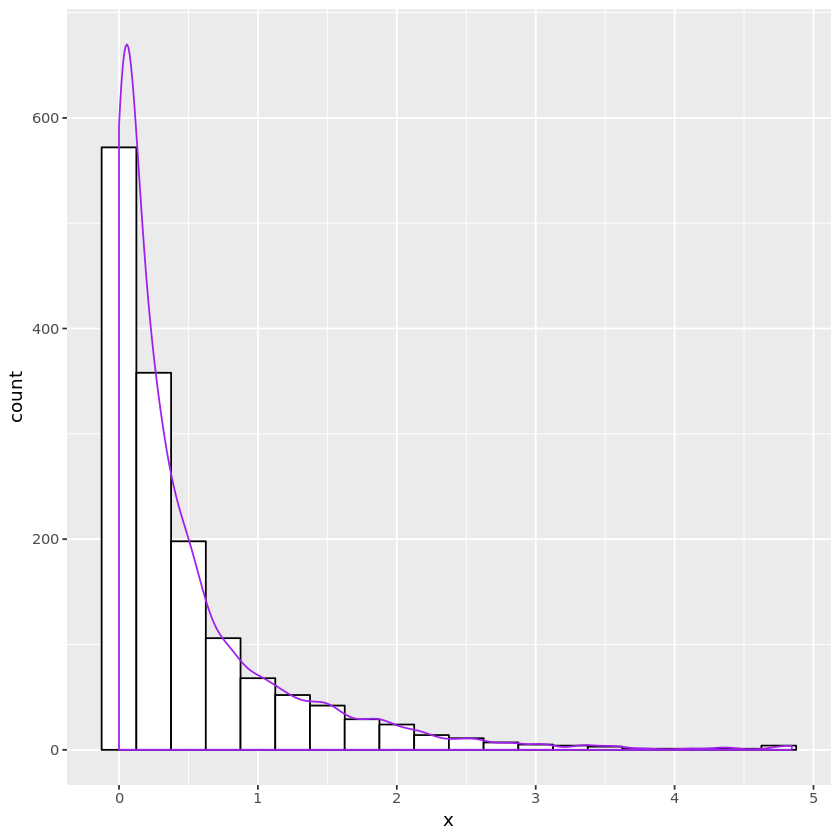
gengamma_ar <- function(nsamp, alph) {
    # sample X from g
    v <- runif(nsamp)  # unif rv for inverse method
    idx <- v > 1 / (1 + alph * exp(-1))
    x <- numeric(nsamp)
    x[idx]  = -log(1 / alph + exp(-1)) - log(1 - v[idx])
    x[!idx] = ((1 + alph * exp(-1)) * v[!idx])^(1 / alph)

    # test acceptance
    u <- runif(nsamp)
    idx2 <- (x > 1)
    accept <- logical(nsamp)
    accept[idx2]  <- (u[idx2] < x[idx2]^(alph - 1))
    accept[!idx2] <- (u[!idx2] < exp(-x[!idx2]))

    x[accept]
}

n <- 2000
alph <- 0.5
x <- gengamma_ar(n, alph)
length(x)
length(x) / n
1501
0.7505
gamma(0.5) / (1 / alph + exp(-1) ) # acceptance ratio
0.748540580270693
gamdata <- data.frame(x = x)
plt <- ggplot(gamdata, aes(x=x)) +
    geom_histogram(binwidth=0.25, fill="white", color="black") +
    geom_density(aes(y=0.25 * ..count..), color="purple")
print(plt)
Multivariate random numbers
Batch methods
Multinomial
Suppose we want to sample $(X_1, \dotsc, X_k) \sim \text{mult}(n, p_1, \dotsc, p_k)$, where $\sum_{i=1}^k p_i = 1$, $\sum_{i=1}^n X_i = n$.
- Method 1: draw $n$ independent realization from pmf $(p_1, \dotsc, p_k)$.
- An easy way is to declare category $j$, $j \in {1, \dotsc, k}$ if \(U \in \left[\sum_{k=0}^{j-1} p_k, \sum_{k=0}^{j} p_k \right),\) where $U \sim \text{unif}[0, 1]$. Take $p_0 = 0$.
- Method 2: sample $k$ independent Poisson random variables $(X_1, \dotsc, X_k)$ with means $\lambda p_1, \dotsc, \lambda p_k$. If the total number of successes $\sum_{i=1}^k X_i$ is equal to $n$, then the conditional distribution of $(X_1, \dotsc, X_k)$ is the desired multinomial.
- We must be fortunate for the sum to be exactly $n$.
Multivariate normal
Suppose we want to sample $\mathbf{X} = (X_1, \dotsc, X_p)$ from MVN $N(\boldsymbol{\mu}, \boldsymbol{\Sigma})$. If we can find $\mathbf{L} \in \mathbb{R}^{p \times p}$ such that $\mathbf{L}^T\mathbf{L} = \boldsymbol{\Sigma}$, then \(\mathbf{L}^T\mathbf{Z} + \boldsymbol{\mu}, \quad \mathbf{Z} \sim N(0, \mathbf{I}_p)\) follows the desired distribution.
-
Random vector $\mathbf{Z}$ consists of $p$ independent standard normal random numbers.
-
Possible choices of $\mathbf{L}$ are:
- Cholesky decomposition of $\boldsymbol{\Sigma}$: $\mathbf{L}$ is lower triangular.
- Matrix square root: if $\mathbf{Q}\boldsymbol{\Lambda}\mathbf{Q}^T$ is a eigenvalue decomposition of $\boldsymbol{\Sigma}$, where $\boldsymbol{\Lambda} = \text{diag}(\lambda_1, \dotsc, \lambda_p)$ with $\lambda_i \ge 0$, then \(\mathbf{L} = \mathbf{Q}\boldsymbol{\Lambda}^{1/2}\mathbf{Q}^T, \quad \boldsymbol{\Lambda}^{1/2} = \text{diag}(\lambda_1^{1/2}, \dotsc, \lambda_p^{1/2}) .\) such a matrix is symmetric and positive semidefinite, and is often denoted by $\boldsymbol{\Sigma}^{1/2}$.
-
For large $p$, finding such a decomposition is challenging.
Multivariate $t$
A multivariate $t$ distribution with degrees of freedom $\nu$, scale matrix $\boldsymbol{\Sigma}$, and location vector $\boldsymbol{\mu}$ is the distribution of the random vector \(\mathbf{T} = \frac{1}{\sqrt{\chi^2_{\nu}/\nu}}\mathbf{X} + \boldsymbol{\mu},\) where $\mathbf{X} \sim N(0, \boldsymbol{\Sigma})$, and $\chi^2_{\nu}$ is the chi-square random variable with $\nu$ degrees of freedom, independent of $\mathbf{X}$.
Sequential sampling
In many cases we can sample a random vector by sampling each component in turn and conditioning:
\begin{align}
p_{X_1, \dotsc, X_p}(x_1, \dotsc, x_p)
&= p_{X_1}(x_1)\prod_{j=2}^p p_{X_j|X_1, \dotsc, X_{j-1}}(x_j | x_1, \dotsc, x_{j-1})
&= p_{X_1}(x_1)p_{X_2|X_1}(x_2|x_1) \prod_{j=3}^p p_{X_j|X_2, \dotsc, X_{j-1}}(x_j | x_1, \dotsc, x_{j-1})
&= \dotsb
\end{align}
Multinomial
| For $(X_1, \dotsc, X_k) \sim \text{mult}(n, p_1, \dotsc, p_k)$, it is immediate to see that $X_1 \sim B(n, p_1)$. Given $X_1 = x_1$, $(X_2, \dotsc, X_k) \sim \text{mult}(n - x_1, p_2 / (1 - p_1), \dotsc, p_k / (1 - p_1) )$. Hence $X_2 | {X_1 = x_1} \sim B(n - x_1, p_2 / (1 - p_1) )$ and so on. |
Multivariate normal
If we want to sample $\mathbf{X} = (X_1, \dotsc, X_p)$ from MVN with mean $\boldsymbol{\mu}=(\mu_1, \dotsc, \mu_p)^T$ and covariance matrix $\boldsymbol{\Sigma} = (\sigma_{ij})$, then note that the first component $X_1 \sim N(\mu_1, \sigma_{11})$. From the conditional distribution formula for multivariate normal, we see that
\((X_2, \dotsc, X_p) | \{X_1 = x_1\}
\sim N(\bar{\boldsymbol{\mu}}, \bar{\boldsymbol{\Sigma}}),
\quad
\bar{\boldsymbol{\mu}} = \boldsymbol{\mu}_2 + \boldsymbol{\Sigma}_{12}^T(x_1 - \mu_1)/\sigma_{11},
~
\bar{\boldsymbol{\Sigma}} = \boldsymbol{\Sigma}_{22} - \boldsymbol{\Sigma}_{12}^T\boldsymbol{\Sigma}_{12}/\sigma_{11}\)
if we partition
\begin{align}
\boldsymbol{\mu} &= (\mu_1, \boldsymbol{\mu}_2)^T
\boldsymbol{\Sigma} &= \begin{bmatrix}
\sigma_{11} & \boldsymbol{\Sigma}_{12}
\boldsymbol{\Sigma}_{12}^T & \boldsymbol{\Sigma}_{22}
\end{bmatrix}
.
\end{align}
Comments